Lab 5 - Python Code#
Authors: Valerie Dube, Erzo Garay, Juan Marcos Guerrero y Matias Villalba
Replication and Data analysis#
# Libraries
import numpy as np
import pandas as pd
import seaborn as sns
import matplotlib.pyplot as plt
import statsmodels.api as sm
import statsmodels.formula.api as smf
import hdmpy as hdm

from sklearn.base import BaseEstimator
from sklearn.pipeline import make_pipeline
from sklearn.preprocessing import StandardScaler
from sklearn.model_selection import KFold, cross_val_predict
from sklearn.linear_model import LassoCV, Lasso
from sklearn.tree import DecisionTreeRegressor
from sklearn.ensemble import GradientBoostingRegressor, RandomForestRegressor
1. Descriptives#
1.1. Descriptive table#
# Import data and see first observations
df = pd.read_csv("../../data/processed_esti.csv")
df.head()
| y | w | gender_female | gender_male | gender_transgender | ethnicgrp_asian | ethnicgrp_black | ethnicgrp_mixed_multiple | ethnicgrp_other | ethnicgrp_white | partners1 | postlaunch | msm | age | imd_decile | |
|---|---|---|---|---|---|---|---|---|---|---|---|---|---|---|---|
| 0 | 1 | 1 | 0 | 1 | 0 | 0 | 0 | 1 | 0 | 0 | 0 | 1 | 0 | 27 | 5 |
| 1 | 0 | 0 | 0 | 1 | 0 | 0 | 0 | 0 | 0 | 1 | 0 | 0 | 0 | 19 | 6 |
| 2 | 0 | 1 | 0 | 1 | 0 | 0 | 1 | 0 | 0 | 0 | 0 | 1 | 0 | 26 | 4 |
| 3 | 0 | 0 | 1 | 0 | 0 | 0 | 0 | 0 | 0 | 1 | 1 | 0 | 0 | 20 | 2 |
| 4 | 1 | 1 | 1 | 0 | 0 | 1 | 0 | 0 | 0 | 0 | 0 | 1 | 0 | 24 | 3 |
df.info()
<class 'pandas.core.frame.DataFrame'>
RangeIndex: 1739 entries, 0 to 1738
Data columns (total 15 columns):
 #   Column                    Non-Null Count  Dtype
---  ------                    --------------  -----
 0   y                         1739 non-null   int64
 1   w                         1739 non-null   int64
 2   gender_female             1739 non-null   int64
 3   gender_male               1739 non-null   int64
 4   gender_transgender        1739 non-null   int64
 5   ethnicgrp_asian           1739 non-null   int64
 6   ethnicgrp_black           1739 non-null   int64
 7   ethnicgrp_mixed_multiple  1739 non-null   int64
 8   ethnicgrp_other           1739 non-null   int64
 9   ethnicgrp_white           1739 non-null   int64
 10  partners1                 1739 non-null   int64
 11  postlaunch                1739 non-null   int64
 12  msm                       1739 non-null   int64
 13  age                       1739 non-null   int64
 14  imd_decile                1739 non-null   int64
dtypes: int64(15)
memory usage: 203.9 KB
control = df[df['w'] == 0].drop('y', axis=1)
treatment = df[df['w'] == 1].drop('y', axis=1)
def get_descriptive_stats(group, column):
    if column == 'age':
        count = group[column].count()
    else:
        count = (group[column] == 1).sum()
    mean = group[column].mean()
    std = group[column].std()
    return count, mean, std

variables = df.columns.drop(['w', 'y'])
control_stats = {var: get_descriptive_stats(control, var) for var in variables}
treatment_stats = {var: get_descriptive_stats(treatment, var) for var in variables}

control_df = pd.DataFrame(control_stats, index=['count', 'mean', 'std']).T
treatment_df = pd.DataFrame(treatment_stats, index=['count', 'mean', 'std']).T

control_df.columns = pd.MultiIndex.from_product([['Control'], control_df.columns])
treatment_df.columns = pd.MultiIndex.from_product([['Treatment'], treatment_df.columns])

combined_df = pd.concat([control_df, treatment_df], axis=1)
formatted_table = combined_df[['Control', 'Treatment']].round(2)

print("Table 1: Descriptive Statistics and Balance\n")
print(formatted_table)
Table 1: Descriptive Statistics and Balance

                         Control              Treatment
                           count   mean   std     count   mean   std
gender_female              475.0   0.58  0.49     541.0   0.59  0.49
gender_male                342.0   0.42  0.49     377.0   0.41  0.49
gender_transgender           1.0   0.00  0.03       3.0   0.00  0.06
ethnicgrp_asian             45.0   0.06  0.23      66.0   0.07  0.26
ethnicgrp_black             76.0   0.09  0.29      74.0   0.08  0.27
ethnicgrp_mixed_multiple    76.0   0.09  0.29      78.0   0.08  0.28
ethnicgrp_other             14.0   0.02  0.13       9.0   0.01  0.10
ethnicgrp_white            607.0   0.74  0.44     694.0   0.75  0.43
partners1                  239.0   0.29  0.46     277.0   0.30  0.46
postlaunch                 387.0   0.47  0.50     512.0   0.56  0.50
msm                        113.0   0.14  0.35     114.0   0.12  0.33
age                        818.0  23.05  3.59     921.0  23.16  3.54
imd_decile                  37.0   3.48  1.49      36.0   3.46  1.47
The observations for each variable are generally balanced between the control and treatment groups. Additionally, most participants are white, with an average age of approximately 23. The mean IMD decile scores are around 3.5, indicating that participants in both groups tend to come from more deprived areas.
1.2. Descriptive graphs#
ax = sns.barplot(
    data=df.groupby('w')['gender_male'].value_counts(normalize=True).to_frame().set_axis(['prop'], axis=1),
    x="gender_male",
    y="prop",
    hue="w",
    )

ax.yaxis.set_major_formatter("{x:.0%}")
ax.set_xlabel("Gender (male=1, female or transgender=0)")
ax.legend(title='')
new_labels = ['Control', 'Treatment']  # Replace with your desired labels
for t, l in zip(ax.get_legend().texts, new_labels):
    t.set_text(l)

plt.show()
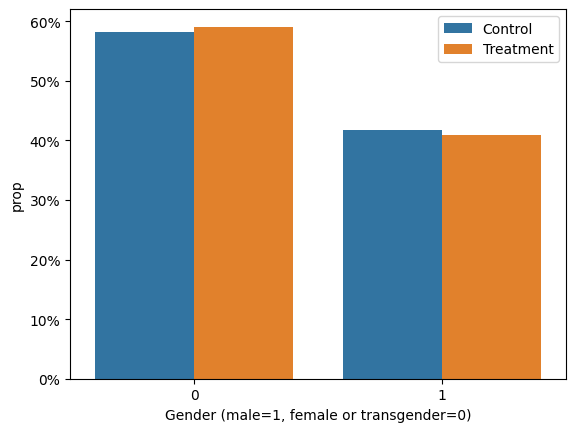
As we saw in section 1.1., there is a similar percentage of males and females participants in each treatment group in the sample.
ax = sns.barplot(
    data=df.groupby('w')['partners1'].value_counts(normalize=True).to_frame().set_axis(['prop'], axis=1),
    x="partners1",
    y="prop",
    hue="w",
    )

ax.yaxis.set_major_formatter("{x:.0%}")
ax.set_xlabel("Number of partners (one partner=1)")
ax.legend(title='')
new_labels = ['Control', 'Treatment']  # Replace with your desired labels
for t, l in zip(ax.get_legend().texts, new_labels):
    t.set_text(l)

plt.show()
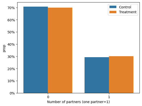
In a similar manner, we note an equal percentage of participants with 2 or more sexual partners as well as those with 1 sexual partner in the last 12 months from the beginning of the study, per treatment or control group.
ax = sns.histplot(data=df, x="age", hue="w", element="poly", stat="percent", common_norm=False)

new_labels = ['Control', 'Treatment']  # Replace with your desired labels
for t, l in zip(ax.get_legend().texts, new_labels):
    t.set_text(l)

plt.show()
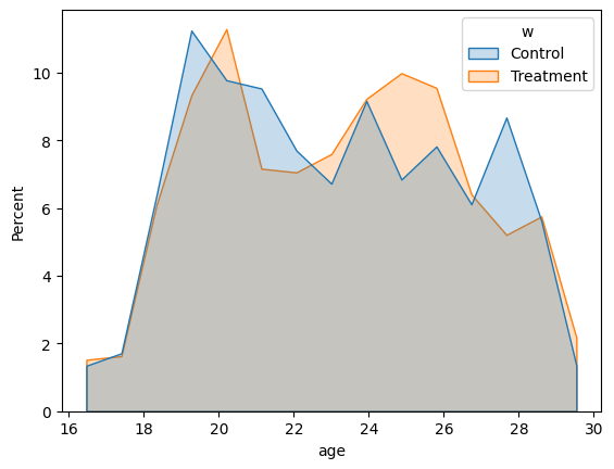
We can see a higher percentage of participants aged between 23 and 27 in the treatment group. Also, there is a higher perceptange of participants aged between 21 and 22 and 27 and 29 in the control group.
ax = sns.histplot(data=df, x="imd_decile", hue="w", element="poly", discrete=True, stat="percent", common_norm=False)

new_labels = ['Control', 'Treatment']  # Replace with your desired labels
for t, l in zip(ax.get_legend().texts, new_labels):
    t.set_text(l)

plt.show()
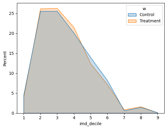
In the case of the IMD decile, an index that measures poverty in the UK, we can see the same proportion of participants in each group.
2. Linear Regression analysis#
2.1. Regression 1: \(y = \beta_0 + \beta_1 T + \epsilon\)#
model_1 = "y ~ w"
est_1 = smf.ols(formula=model_1 , data=df).fit()

print(est_1.summary())
                            OLS Regression Results
==============================================================================
Dep. Variable:                      y   R-squared:                       0.077
Model:                            OLS   Adj. R-squared:                  0.076
Method:                 Least Squares   F-statistic:                     144.5
Date:                Wed, 07 Aug 2024   Prob (F-statistic):           4.96e-32
Time:                        21:44:28   Log-Likelihood:                -1112.9
No. Observations:                1739   AIC:                             2230.
Df Residuals:                    1737   BIC:                             2241.
Df Model:                           1
Covariance Type:            nonrobust
==============================================================================
                 coef    std err          t      P>|t|      [0.025      0.975]
------------------------------------------------------------------------------
Intercept      0.2115      0.016     13.174      0.000       0.180       0.243
w              0.2652      0.022     12.021      0.000       0.222       0.308
==============================================================================
Omnibus:                    38241.926   Durbin-Watson:                   1.995
Prob(Omnibus):                  0.000   Jarque-Bera (JB):              217.327
Skew:                           0.532   Prob(JB):                     6.43e-48
Kurtosis:                       1.634   Cond. No.                         2.69
==============================================================================

Notes:
[1] Standard Errors assume that the covariance matrix of the errors is correctly specified.
We found that the adjusted R-squared is 0.076 and the ATE is approximately 0.27. This means that the treatment explains only 7.6% of the increase in the STI tests between the control and treatment groups. Additionally, receiving the treatment (i.e. being invited to use the internet-based sexual health service) increases, on average, the probability of taking an STI test by 26.5%.
2.2. Regression 2: \(y = \beta_0 + \beta_1 T + \beta_2 X + \epsilon\)#
model_2 = "y ~ w + age + gender_female + ethnicgrp_white + ethnicgrp_black + ethnicgrp_mixed_multiple + partners1 + imd_decile + msm"
est_2 = smf.ols(formula=model_2 , data=df).fit()

print(est_2.summary())
                            OLS Regression Results
==============================================================================
Dep. Variable:                      y   R-squared:                       0.107
Model:                            OLS   Adj. R-squared:                  0.102
Method:                 Least Squares   F-statistic:                     22.94
Date:                Wed, 07 Aug 2024   Prob (F-statistic):           3.06e-37
Time:                        21:44:28   Log-Likelihood:                -1084.3
No. Observations:                1739   AIC:                             2189.
Df Residuals:                    1729   BIC:                             2243.
Df Model:                           9
Covariance Type:            nonrobust
============================================================================================
                               coef    std err          t      P>|t|      [0.025      0.975]
--------------------------------------------------------------------------------------------
Intercept                   -0.1807      0.088     -2.042      0.041      -0.354      -0.007
w                            0.2622      0.022     12.044      0.000       0.220       0.305
age                          0.0149      0.003      4.787      0.000       0.009       0.021
gender_female                0.0905      0.025      3.629      0.000       0.042       0.139
ethnicgrp_white              0.0499      0.041      1.209      0.227      -0.031       0.131
ethnicgrp_black             -0.0292      0.054     -0.538      0.591      -0.136       0.077
ethnicgrp_mixed_multiple    -0.0315      0.054     -0.587      0.557      -0.137       0.074
partners1                   -0.0661      0.024     -2.714      0.007      -0.114      -0.018
imd_decile                  -0.0045      0.007     -0.609      0.543      -0.019       0.010
msm                          0.0033      0.037      0.089      0.929      -0.069       0.075
==============================================================================
Omnibus:                     2495.421   Durbin-Watson:                   1.997
Prob(Omnibus):                  0.000   Jarque-Bera (JB):              193.943
Skew:                           0.524   Prob(JB):                     7.69e-43
Kurtosis:                       1.743   Cond. No.                         215.
==============================================================================

Notes:
[1] Standard Errors assume that the covariance matrix of the errors is correctly specified.
Compared to the previous regression, when we include additional variables (age, gender, ethnic group, number of sexual partners, the indicator for Randomised after SH:24 made publicly available, the indicator for men who have sex with men, and the socioeconomic level measured by deciles), we observe an increase in the adjusted R-squared of approximately 0.3 percentage points (from 0.1). Additionally, the ATE decreases by 0.003 percentage points, indicating a negative bias.
It is worth mentioning that we omit gender_male to avoid collinearity with gender_female. Similarly, we exclude the less relevant ethnic group (i.e. the one with fewer observations) to prevent the same issue.
2.3. Regression 3: \(y = \beta_0 + \beta_1 T + \beta_2 X + \epsilon\) (Double Lasso variable selection)#
# Assuming df is already defined
X = df[["gender_female", "ethnicgrp_white", "ethnicgrp_black", "gender_transgender", "msm", "partners1", "age", "imd_decile"]]
w = df['w']
y = df['y']

# Fit LassoCV model to find the optimal alpha (lambda)
cv_model3a = LassoCV(alphas=None, cv=10, max_iter=10000).fit(X, w)
cv_model3b = LassoCV(alphas=None, cv=10, max_iter=10000).fit(X, y)

# Fit Lasso model with the optimal alpha
model3a = Lasso(alpha=cv_model3a.alpha_).fit(X, w)
model3b = Lasso(alpha=cv_model3b.alpha_).fit(X, y)

# Identify non-zero coefficients from Lasso models
significant_vars3a = X.columns[model3a.coef_ != 0]
significant_vars3b = X.columns[model3b.coef_ != 0]

# Combine the significant variables from both models
significant_vars = pd.Index(np.unique(significant_vars3a.append(significant_vars3b)))

# Extract the significant variables for regression
X_significant = X[significant_vars]

# Add 'w' to the significant variables
X_significant_with_w = X_significant.copy()
X_significant_with_w['w'] = w

# Add constant term for intercept in the new significant variable set
X_significant_with_w = sm.add_constant(X_significant_with_w)

# Fit linear regression model on significant variables plus 'w' against 'y'
model3 = sm.OLS(y, X_significant_with_w).fit()

# Print summary of the model
print("Summary for the final model with dependent variable 'y':")
print(model3.summary())
Summary for the final model with dependent variable 'y':
                            OLS Regression Results
==============================================================================
Dep. Variable:                      y   R-squared:                       0.106
Model:                            OLS   Adj. R-squared:                  0.103
Method:                 Least Squares   F-statistic:                     34.38
Date:                Wed, 07 Aug 2024   Prob (F-statistic):           2.06e-39
Time:                        21:44:28   Log-Likelihood:                -1084.5
No. Observations:                1739   AIC:                             2183.
Df Residuals:                    1732   BIC:                             2221.
Df Model:                           6
Covariance Type:            nonrobust
===================================================================================
                      coef    std err          t      P>|t|      [0.025      0.975]
-----------------------------------------------------------------------------------
const              -0.2026      0.081     -2.508      0.012      -0.361      -0.044
age                 0.0149      0.003      4.824      0.000       0.009       0.021
ethnicgrp_white     0.0710      0.025      2.805      0.005       0.021       0.121
gender_female       0.0888      0.022      3.977      0.000       0.045       0.133
imd_decile         -0.0042      0.007     -0.569      0.570      -0.019       0.010
partners1          -0.0660      0.024     -2.725      0.006      -0.114      -0.019
w                   0.2626      0.022     12.078      0.000       0.220       0.305
==============================================================================
Omnibus:                     2501.289   Durbin-Watson:                   1.996
Prob(Omnibus):                  0.000   Jarque-Bera (JB):              194.167
Skew:                           0.524   Prob(JB):                     6.87e-43
Kurtosis:                       1.743   Cond. No.                         177.
==============================================================================

Notes:
[1] Standard Errors assume that the covariance matrix of the errors is correctly specified.
We observe that the ATE using double lasso is akin to the OLS with confounders, along with the adjusted R-squared.
2.4. Coefficient Comparison#
# Assuming model1, model2, model3 are your fitted statsmodels regression models
# Extract the coefficients for resW
b1 = est_1.params['w']
b2 = est_2.params['w']
b3 = model3.params['w']

# Extract the standard errors for resW
se1 = est_1.bse['w']
se2 = est_2.bse['w']
se3 = model3.bse['w']

# Labels for the models
model_labels = ['OLS', 'OLS w. controls', 'Double Lasso']

# Coefficients and standard errors
coefficients = [b1, b2, b3]
errors = [se1, se2, se3]

# Create the figure and axis
fig, ax = plt.subplots()

# Plot the coefficients with error bars
ax.errorbar(model_labels, coefficients, yerr=errors, fmt='o', capsize=5, capthick=2, marker='s', markersize=7, linestyle='None')

# Add title and labels
ax.set_title('Comparison of Coefficients from Different Models')
ax.set_xlabel('Model')
ax.set_ylabel('Coefficient')

# Add grid for better readability
ax.grid(True)

# Show the plot
plt.show()
C:\Users\Matias Villalba\AppData\Local\Temp\ipykernel_10508\2861833790.py:23: UserWarning: marker is redundantly defined by the 'marker' keyword argument and the fmt string "o" (-> marker='o'). The keyword argument will take precedence.
  ax.errorbar(model_labels, coefficients, yerr=errors, fmt='o', capsize=5, capthick=2, marker='s', markersize=7, linestyle='None')
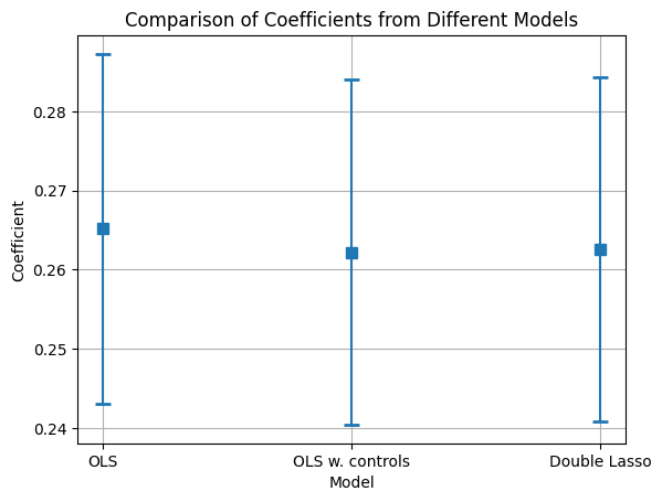
In general, the three ATEs are very similar, but we consider that the models that include the cofounders (OLS with controls and DL) are better estimated.
3. Non-Linear Methods DML#
def dml(X, D, y, modely, modeld, *, nfolds, classifier=False, time = None, clu = None, cluster = True):
    cv = KFold(n_splits=nfolds, shuffle=True, random_state=123) # shuffled k-folds
    yhat = cross_val_predict(modely, X, y, cv=cv, n_jobs=-1) # out-of-fold predictions for y
    # out-of-fold predictions for D
    # use predict or predict_proba dependent on classifier or regressor for D
    if classifier:
        Dhat = cross_val_predict(modeld, X, D, cv=cv, method='predict_proba', n_jobs=-1)[:, 1]
    else:
        Dhat = cross_val_predict(modeld, X, D, cv=cv, n_jobs=-1)
    # calculate outcome and treatment residuals
    resy = y - yhat
    resD = D - Dhat

    if cluster:
      # final stage ols clustered
      dml_data = pd.concat([clu, pd.Series(time), pd.Series(resy, name = 'resy'), pd.Series(resD, name = 'resD')], axis=1)

    else:
      # final stage ols nonclustered
      dml_data = pd.concat([pd.Series(resy, name = 'resy'), pd.Series(resD, name = 'resD')], axis=1)

    if cluster:
      # clustered standard errors
      ols_mod = smf.ols(formula = 'resy ~ 1 + resD', data = dml_data).fit(cov_type='cluster', cov_kwds={"groups": dml_data['CountyCode']})

    else:
      # regular ols
      ols_mod = smf.ols(formula = 'resy ~ 1 + resD', data = dml_data).fit()

    point = ols_mod.params[1]
    stderr = ols_mod.bse[1]
    epsilon = ols_mod.resid

    return point, stderr, yhat, Dhat, resy, resD, epsilon
def summary(point, stderr, yhat, Dhat, resy, resD, epsilon, X, D, y, *, name):
    '''
    Convenience summary function that takes the results of the DML function
    and summarizes several estimation quantities and performance metrics.
    '''
    return pd.DataFrame({'estimate': point, # point estimate
                         'stderr': stderr, # standard error
                         'lower': point - 1.96*stderr, # lower end of 95% confidence interval
                         'upper': point + 1.96*stderr, # upper end of 95% confidence interval
                         'rmse y': np.sqrt(np.mean(resy**2)), # RMSE of model that predicts outcome y
                         'rmse D': np.sqrt(np.mean(resD**2)) # RMSE of model that predicts treatment D
                         }, index=[name])
df['intercept'] = 1
y = df["y"]
d = df["w"]
x = df[df.columns[~df.columns.isin(['y','w'])]]
3.1. DML with RLasso#
class RLasso(BaseEstimator):

    def __init__(self, *, post=True):
        self.post = post

    def fit(self, X, y):
        self.rlasso_ = hdmpy.rlasso(X, y, post=self.post)
        return self

    def predict(self, X):
        return np.array(X) @ np.array(self.rlasso_.est['beta']).flatten() + np.array(self.rlasso_.est['intercept'])

lasso_model = lambda: RLasso(post=False)
# DML with RLasso:
modely = make_pipeline(StandardScaler(), RLasso(post=False))
modeld = make_pipeline(StandardScaler(), RLasso(post=False))
result_RLasso = dml(x,d,y, modely, modeld, nfolds=10, classifier=False, cluster = False)
table_RLasso = summary(*result_RLasso, x,d,y, name = 'Lasso')
print(table_RLasso)
---------------------------------------------------------------------------
_RemoteTraceback                          Traceback (most recent call last)
_RemoteTraceback:
"""
Traceback (most recent call last):
  File "C:\Users\Matias Villalba\AppData\Local\Programs\Python\Python312\Lib\site-packages\joblib\externals\loky\process_executor.py", line 463, in _process_worker
    r = call_item()
        ^^^^^^^^^^^
  File "C:\Users\Matias Villalba\AppData\Local\Programs\Python\Python312\Lib\site-packages\joblib\externals\loky\process_executor.py", line 291, in __call__
    return self.fn(*self.args, **self.kwargs)
           ^^^^^^^^^^^^^^^^^^^^^^^^^^^^^^^^^^
  File "C:\Users\Matias Villalba\AppData\Local\Programs\Python\Python312\Lib\site-packages\joblib\parallel.py", line 598, in __call__
    return [func(*args, **kwargs)
            ^^^^^^^^^^^^^^^^^^^^^
  File "C:\Users\Matias Villalba\AppData\Local\Programs\Python\Python312\Lib\site-packages\sklearn\utils\parallel.py", line 129, in __call__
    return self.function(*args, **kwargs)
           ^^^^^^^^^^^^^^^^^^^^^^^^^^^^^^
  File "C:\Users\Matias Villalba\AppData\Local\Programs\Python\Python312\Lib\site-packages\sklearn\model_selection\_validation.py", line 1378, in _fit_and_predict
    estimator.fit(X_train, y_train, **fit_params)
  File "C:\Users\Matias Villalba\AppData\Local\Programs\Python\Python312\Lib\site-packages\sklearn\base.py", line 1474, in wrapper
    return fit_method(estimator, *args, **kwargs)
           ^^^^^^^^^^^^^^^^^^^^^^^^^^^^^^^^^^^^^^
  File "C:\Users\Matias Villalba\AppData\Local\Programs\Python\Python312\Lib\site-packages\sklearn\pipeline.py", line 475, in fit
    self._final_estimator.fit(Xt, y, **last_step_params["fit"])
  File "C:\Users\Matias Villalba\AppData\Local\Temp\ipykernel_10508\3396256270.py", line 7, in fit
NameError: name 'hdmpy' is not defined
"""

The above exception was the direct cause of the following exception:

NameError                                 Traceback (most recent call last)
Cell In[19], line 4
      2 modely = make_pipeline(StandardScaler(), RLasso(post=False))
      3 modeld = make_pipeline(StandardScaler(), RLasso(post=False))
----> 4 result_RLasso = dml(x,d,y, modely, modeld, nfolds=10, classifier=False, cluster = False)
      5 table_RLasso = summary(*result_RLasso, x,d,y, name = 'Lasso')
      6 print(table_RLasso)

Cell In[15], line 3, in dml(X, D, y, modely, modeld, nfolds, classifier, time, clu, cluster)
      1 def dml(X, D, y, modely, modeld, *, nfolds, classifier=False, time = None, clu = None, cluster = True):
      2     cv = KFold(n_splits=nfolds, shuffle=True, random_state=123) # shuffled k-folds
----> 3     yhat = cross_val_predict(modely, X, y, cv=cv, n_jobs=-1) # out-of-fold predictions for y
      4     # out-of-fold predictions for D
      5     # use predict or predict_proba dependent on classifier or regressor for D
      6     if classifier:

File ~\AppData\Local\Programs\Python\Python312\Lib\site-packages\sklearn\utils\_param_validation.py:213, in validate_params.<locals>.decorator.<locals>.wrapper(*args, **kwargs)
    207 try:
    208     with config_context(
    209         skip_parameter_validation=(
    210             prefer_skip_nested_validation or global_skip_validation
    211         )
    212     ):
--> 213         return func(*args, **kwargs)
    214 except InvalidParameterError as e:
    215     # When the function is just a wrapper around an estimator, we allow
    216     # the function to delegate validation to the estimator, but we replace
    217     # the name of the estimator by the name of the function in the error
    218     # message to avoid confusion.
    219     msg = re.sub(
    220         r"parameter of \w+ must be",
    221         f"parameter of {func.__qualname__} must be",
    222         str(e),
    223     )

File ~\AppData\Local\Programs\Python\Python312\Lib\site-packages\sklearn\model_selection\_validation.py:1293, in cross_val_predict(estimator, X, y, groups, cv, n_jobs, verbose, fit_params, params, pre_dispatch, method)
   1290 # We clone the estimator to make sure that all the folds are
   1291 # independent, and that it is pickle-able.
   1292 parallel = Parallel(n_jobs=n_jobs, verbose=verbose, pre_dispatch=pre_dispatch)
-> 1293 predictions = parallel(
   1294     delayed(_fit_and_predict)(
   1295         clone(estimator),
   1296         X,
   1297         y,
   1298         train,
   1299         test,
   1300         routed_params.estimator.fit,
   1301         method,
   1302     )
   1303     for train, test in splits
   1304 )
   1306 inv_test_indices = np.empty(len(test_indices), dtype=int)
   1307 inv_test_indices[test_indices] = np.arange(len(test_indices))

File ~\AppData\Local\Programs\Python\Python312\Lib\site-packages\sklearn\utils\parallel.py:67, in Parallel.__call__(self, iterable)
     62 config = get_config()
     63 iterable_with_config = (
     64     (_with_config(delayed_func, config), args, kwargs)
     65     for delayed_func, args, kwargs in iterable
     66 )
---> 67 return super().__call__(iterable_with_config)

File ~\AppData\Local\Programs\Python\Python312\Lib\site-packages\joblib\parallel.py:2007, in Parallel.__call__(self, iterable)
   2001 # The first item from the output is blank, but it makes the interpreter
   2002 # progress until it enters the Try/Except block of the generator and
   2003 # reach the first `yield` statement. This starts the aynchronous
   2004 # dispatch of the tasks to the workers.
   2005 next(output)
-> 2007 return output if self.return_generator else list(output)

File ~\AppData\Local\Programs\Python\Python312\Lib\site-packages\joblib\parallel.py:1650, in Parallel._get_outputs(self, iterator, pre_dispatch)
   1647     yield
   1649     with self._backend.retrieval_context():
-> 1650         yield from self._retrieve()
   1652 except GeneratorExit:
   1653     # The generator has been garbage collected before being fully
   1654     # consumed. This aborts the remaining tasks if possible and warn
   1655     # the user if necessary.
   1656     self._exception = True

File ~\AppData\Local\Programs\Python\Python312\Lib\site-packages\joblib\parallel.py:1754, in Parallel._retrieve(self)
   1747 while self._wait_retrieval():
   1748
   1749     # If the callback thread of a worker has signaled that its task
   1750     # triggered an exception, or if the retrieval loop has raised an
   1751     # exception (e.g. `GeneratorExit`), exit the loop and surface the
   1752     # worker traceback.
   1753     if self._aborting:
-> 1754         self._raise_error_fast()
   1755         break
   1757     # If the next job is not ready for retrieval yet, we just wait for
   1758     # async callbacks to progress.

File ~\AppData\Local\Programs\Python\Python312\Lib\site-packages\joblib\parallel.py:1789, in Parallel._raise_error_fast(self)
   1785 # If this error job exists, immediatly raise the error by
   1786 # calling get_result. This job might not exists if abort has been
   1787 # called directly or if the generator is gc'ed.
   1788 if error_job is not None:
-> 1789     error_job.get_result(self.timeout)

File ~\AppData\Local\Programs\Python\Python312\Lib\site-packages\joblib\parallel.py:745, in BatchCompletionCallBack.get_result(self, timeout)
    739 backend = self.parallel._backend
    741 if backend.supports_retrieve_callback:
    742     # We assume that the result has already been retrieved by the
    743     # callback thread, and is stored internally. It's just waiting to
    744     # be returned.
--> 745     return self._return_or_raise()
    747 # For other backends, the main thread needs to run the retrieval step.
    748 try:

File ~\AppData\Local\Programs\Python\Python312\Lib\site-packages\joblib\parallel.py:763, in BatchCompletionCallBack._return_or_raise(self)
    761 try:
    762     if self.status == TASK_ERROR:
--> 763         raise self._result
    764     return self._result
    765 finally:

NameError: name 'hdmpy' is not defined
The message treatment providing information about Internet-accessed sexually transmitted infection testing predicts an increase in the probability that a person will get tested by 25.91 percentage points compared to receiving information about nearby clinics offering in-person testing. By providing both groups with information about testing, we mitigate the potential reminder effect, as both groups are equally prompted to consider testing. This approach allows us to isolate the impact of the type of information “Internet-accessed testing” versus “in-person clinic testing” on the likelihood of getting tested. Through randomized assignment, we establish causality rather than mere correlation, confirming that the intervention’s effect is driven by the unique advantages of Internet-accessed testing, such as increased privacy, reduced embarrassment, and convenience
3.2. DML with Regression Trees#
modely = make_pipeline(StandardScaler(), DecisionTreeRegressor(ccp_alpha=0.001, min_samples_leaf=5, random_state=123))
modeld = make_pipeline(StandardScaler(), DecisionTreeRegressor(ccp_alpha=0.001, min_samples_leaf=5, random_state=123))
result_RT = dml(x,d,y, modely, modeld, nfolds=10, classifier=False, cluster = False)
table_RT= summary(*result_RT, x,d,y, name = 'RT')
print(table_RT)
    estimate    stderr     lower     upper    rmse y    rmse D
RT  0.249831  0.021872  0.206961  0.292701  0.472259  0.499638
C:\Users\Matias Villalba\AppData\Local\Temp\ipykernel_23460\2498640246.py:30: FutureWarning: Series.__getitem__ treating keys as positions is deprecated. In a future version, integer keys will always be treated as labels (consistent with DataFrame behavior). To access a value by position, use `ser.iloc[pos]`
  point = ols_mod.params[1]
C:\Users\Matias Villalba\AppData\Local\Temp\ipykernel_23460\2498640246.py:31: FutureWarning: Series.__getitem__ treating keys as positions is deprecated. In a future version, integer keys will always be treated as labels (consistent with DataFrame behavior). To access a value by position, use `ser.iloc[pos]`
  stderr = ols_mod.bse[1]
The message treatment providing information about Internet-accessed sexually transmitted infection testing predicts an increase in the probability that a person will get tested by 24.98 percentage points compared to receiving information about nearby clinics offering in-person testing. By providing both groups with information about testing, we mitigate the potential reminder effect, as both groups are equally prompted to consider testing. This approach allows us to isolate the impact of the type of information “Internet-accessed testing” versus “in-person clinic testing” on the likelihood of getting tested. Through randomized assignment, we establish causality rather than mere correlation, confirming that the intervention’s effect is driven by the unique advantages of Internet-accessed testing, such as increased privacy, reduced embarrassment, and convenience
3.3. DML Boosting Trees#
modely = make_pipeline(StandardScaler(), GradientBoostingRegressor(n_estimators=100, max_depth=3, random_state=123))
modeld = make_pipeline(StandardScaler(), GradientBoostingRegressor(n_estimators=100, max_depth=3, random_state=123))
result_GBT = dml(x,d,y, modely, modeld, nfolds=10, classifier=False, cluster = False)
table_GBT = summary(*result_GBT, x,d,y, name = 'GBT')
print(table_GBT)
     estimate    stderr     lower     upper    rmse y    rmse D
GBT  0.246373  0.021669  0.203902  0.288843  0.475893  0.508383
C:\Users\Matias Villalba\AppData\Local\Temp\ipykernel_23460\2498640246.py:30: FutureWarning: Series.__getitem__ treating keys as positions is deprecated. In a future version, integer keys will always be treated as labels (consistent with DataFrame behavior). To access a value by position, use `ser.iloc[pos]`
  point = ols_mod.params[1]
C:\Users\Matias Villalba\AppData\Local\Temp\ipykernel_23460\2498640246.py:31: FutureWarning: Series.__getitem__ treating keys as positions is deprecated. In a future version, integer keys will always be treated as labels (consistent with DataFrame behavior). To access a value by position, use `ser.iloc[pos]`
  stderr = ols_mod.bse[1]
The message treatment providing information about Internet-accessed sexually transmitted infection testing predicts an increase in the probability that a person will get tested by 24.64 percentage points compared to receiving information about nearby clinics offering in-person testing. By providing both groups with information about testing, we mitigate the potential reminder effect, as both groups are equally prompted to consider testing. This approach allows us to isolate the impact of the type of information “Internet-accessed testing” versus “in-person clinic testing” on the likelihood of getting tested. Through randomized assignment, we establish causality rather than mere correlation, confirming that the intervention’s effect is driven by the unique advantages of Internet-accessed testing, such as increased privacy, reduced embarrassment, and convenience
3.4. DML with Random Forest#
modely = make_pipeline(StandardScaler(), RandomForestRegressor(n_estimators=100, min_samples_leaf=5, random_state=123))
modeld = make_pipeline(StandardScaler(), RandomForestRegressor(n_estimators=100, min_samples_leaf=5, random_state=123))
result_RF = dml(x,d,y, modely, modeld, nfolds=10, classifier=False, cluster = False)
table_RF = summary(*result_RF, x,d,y, name = 'RF')
print(table_RF)
    estimate    stderr     lower     upper    rmse y    rmse D
RF  0.241558  0.021379  0.199655  0.283461  0.472297  0.511585
C:\Users\Matias Villalba\AppData\Local\Temp\ipykernel_23460\2498640246.py:30: FutureWarning: Series.__getitem__ treating keys as positions is deprecated. In a future version, integer keys will always be treated as labels (consistent with DataFrame behavior). To access a value by position, use `ser.iloc[pos]`
  point = ols_mod.params[1]
C:\Users\Matias Villalba\AppData\Local\Temp\ipykernel_23460\2498640246.py:31: FutureWarning: Series.__getitem__ treating keys as positions is deprecated. In a future version, integer keys will always be treated as labels (consistent with DataFrame behavior). To access a value by position, use `ser.iloc[pos]`
  stderr = ols_mod.bse[1]
The message treatment providing information about Internet-accessed sexually transmitted infection testing predicts an increase in the probability that a person will get tested by 24.16 percentage points compared to receiving information about nearby clinics offering in-person testing. By providing both groups with information about testing, we mitigate the potential reminder effect, as both groups are equally prompted to consider testing. This approach allows us to isolate the impact of the type of information “Internet-accessed testing” versus “in-person clinic testing” on the likelihood of getting tested. Through randomized assignment, we establish causality rather than mere correlation, confirming that the intervention’s effect is driven by the unique advantages of Internet-accessed testing, such as increased privacy, reduced embarrassment, and convenience
3.6.#
# Extract coefficients and standard errors
coefficients = [result_RLasso[0], result_RT[0], result_GBT[0], result_RF[0]]
standard_errors = [result_RLasso[1], result_RT[1], result_GBT[1], result_RF[1]]
methods = ['RLasso', 'Regression Trees', 'Boosting Trees', 'Regression Forest']
# Plotting the coefficients with error bars
plt.figure(figsize=(10, 6))
plt.errorbar(methods, coefficients, yerr=standard_errors, fmt='o', capsize=5, capthick=2)
plt.xlabel('Regression Methods')
plt.ylabel('Coefficients')
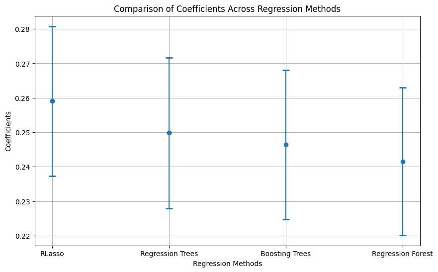
plt.title('Comparison of Coefficients Across Regression Methods')
plt.grid(True)
plt.show()
results_table = pd.concat([table_RLasso, table_RT, table_GBT, table_RF], axis=0)
print(results_table)
       estimate    stderr     lower     upper    rmse y    rmse D
Lasso  0.259067  0.021722  0.216492  0.301642  0.471041  0.500225
RT     0.249831  0.021872  0.206961  0.292701  0.472259  0.499638
GBT    0.246373  0.021669  0.203902  0.288843  0.475893  0.508383
RF     0.241558  0.021379  0.199655  0.283461  0.472297  0.511585
To choose the best model, we must compare the RMSEs of the outcome variable Y. In this case, the model with the lowest RMSE for Y is generated by Lasso (0.471041), whereas the lowest for the treatment is generated by Regression Trees (0.4983734). Therefore, DML could be employed with Y cleaned using Lasso and the treatment using Regression Trees.