Lab 3 - Python Code#
Group 3: Valerie Dube, Erzo Garay, Juan Marcos Guerrero y Matías Villalba,
1. Neyman Orthogonality Proof#
\(Y_{nx1}=\alpha D_{nx1}+W_{nxp}\beta_{px1}+\epsilon_{nx1}\\ \widetilde{Y}_{nx1}=Y_{nx1}-W_{nxp}X_{{{Yw}_{px1}}}\\ \widetilde{D}_{nx1}=D_{nx1}-W_{nxp}X_{{{Dw}_{px1}}}\\ W=Matrix\ composed\ by\ one\ variable\ in\ each\ column\\ X=Vector\ of\ coefficients\\ n=N° observations\\ p=N° confounders \\\ \\\ \\\ M(a,\eta)=E[(\widetilde{Y}_{nx1}(\eta_{1})-a\widetilde{D}(\eta_{2})_{nx1})'(\widetilde{D}(\eta_{2})_{nx1})]=0\\ \frac{\partial a}{\partial \eta}=-[\frac{\partial M}{\partial a}(\alpha,\eta_{0})]^{-1}[\frac{\partial M}{\partial \eta}(\alpha,\eta_{0})]\\ \frac{\partial M}{\partial \eta}(\alpha,\eta_{0})=\frac{\partial M}{\partial \eta_{1}}(\alpha,X_{Yw},X_{Dw})+\frac{\partial M}{\partial \eta_{2}}(\alpha,X_{Yw},X_{Dw})\\ S_{1}=\frac{\partial M}{\partial \eta_{1}}(\alpha,X_{Yw},X_{Dw}) , S_{2}=\frac{\partial M}{\partial \eta_{2}}(\alpha,X_{Yw},X_{Dw})\)
Demonstration 1:#
\(Given\ the\ general\ formula\,\ before\ using\ (\alpha,X_{Yw},X_{Dw}): \widetilde{Y}_{nx1}=Y_{nx1}-W_{nxp}\eta_{{{1}_{px1}}} ,\ \widetilde{D}_{nx1}=D_{nx1}-W_{nxp}\eta_{{{2}_{px1}}}: \\\ \\\ S_{1}=\frac{\partial M}{\partial \eta_{1}}|_{(\alpha,W_{Yw},W_{Dw})}\\\ \\\ =\frac{\partial E[(\widetilde{Y}_{nx1}(\eta_{1})-a\widetilde{D}(\eta_{2})_{nx1})'(\widetilde{D}(\eta_{2})_{nx1})}{\partial \eta_{1}}|_{(\alpha,W_{Yw},W_{Dw})}=\frac{\partial E[Y_{nx1}-W_{nxp}\eta_{{{1}_{px1}}}-aD_{nx1}+aW_{nxp}\eta_{{{2}_{px1}}})'(D_{nx1}-W_{nxp}\eta_{{{2}_{px1}}})}{\partial \eta_{1}}|_{(\alpha,W_{Yw},W_{Dw})}\\\ \\\ Substituting\ (\alpha,W_{Yw},W_{Dw})\ in\ (a,\eta_{1},\eta_{2})\\\ \\\ =\frac{\partial E[(\widetilde{Y}_{nx1}(\eta_{1})-a\widetilde{D}(\eta_{2})_{nx1})'(\widetilde{D}(\eta_{2})_{nx1})]}{\partial \eta_{1}}|_{(\alpha,W_{Yw},W_{Dw})}=E[(W_{nxp})'(D_{nx1}-W_{n*p}\eta_{{2}_{px1}})]|_{(\alpha,W_{Yw},W_{Dw})}\\ =E[(W_{nxp})'(D_{nx1}-W_{n*p}X_{{{Dw}_{px1}}})]\\ =E[W'_{pxn}D_{nx1}-W'_{pxn}W_{nxp}(W'_{pxn}W_{nxp})^{-1}(W'_{pxn}D_{nx1})]\\ =E[W'_{pxn}D_{nx1}-I_{pxp}(W'_{pxn}D_{nx1})]=E[W'_{pxn}D_{nx1}-W'_{pxn}D_{nx1}]=E[0]\\ S_{1}=0\)
Demonstration 2:#
\(Given\ the\ general\ formula\,\ before\ using\ (\alpha,X_{Yw},X_{Dw}): \widetilde{Y}_{nx1}=y_{nx1}-W_{nxp}\eta_{{{1}_{px1}}} ,\ \widetilde{D}_{nx1}=D_{nx1}-W_{nxp}\eta_{{{2}_{px1}}}\\\ \\\ S_{2}=\frac{\partial M}{\partial \eta_{2}}|_{(\alpha,W_{Yw},W_{Dw})}=0\\\ \\ =\frac{\partial E[(\widetilde{Y}_{nx1}(\eta_{1})-a\widetilde{D}(\eta_{2})_{nx1})'(\widetilde{D}(\eta_{2})_{nx1})}{\partial \eta_{2}}|_{(\alpha,W_{Yw},W_{Dw})}=\frac{\partial E[Y_{nx1}-W_{nxp}\eta_{{{1}_{px1}}}-aD_{nx1}+aW_{nxp}\eta_{{{2}_{px1}}})'(D_{nx1}-W_{nxp}\eta_{{{2}_{px1}}})}{\partial \eta_{2}}|_{(\alpha,W_{Yw},W_{Dw})}\\ =\frac{\partial E[-Y_{1xn}'W_{nxp}\eta_{{2}_{px1}}+\eta'_{{1}_{1xn}}W'_{pxn}W_{pxn}\eta_{{2}_{px1}}+aD'_{1xn}W_{nxp}\eta_{{2}_{px1}}+a\eta'_{{2}_{1xp}}W'_{pxn}D_{nx1}-a\eta'_{{2}_{1xp}}W'_{pxn}W_{nxp}\eta_{{2}_{px1}}]}{\partial \eta_{2}}|_{(\alpha,W_{Yw},W_{Dw})}\\ =E[-W'_{pxn}Y_{nx1}+W'_{pxn}W_{nxp}\eta_{{1}_{px1}}+aW'_{pxn}D_{nx1}+aW'_{pxn}D_{nx1}-aW'_{pxn}W_{nxp}\eta_{{2}_{px1}}-aW'_{pxn}W_{nxp}\eta_{{2}_{px1}}]|_{(\alpha,W_{Yw},W_{Dw})}\\\ \\\ Substituting\ (\alpha,W_{Yw},W_{Dw})\ in\ (a,\eta_{1},\eta_{2})\\\ \\ =E[-W'_{pxn}Y_{nx1}+W'_{pxn}W_{nxp}X_{{{yw}_{px1}}}+\alpha W'_{pxn}D_{nx1}+\alpha W'_{pxn}D_{nx1}-\alpha W'_{pxn}W_{nxp}X_{{{Dw}_{px1}}}-\alpha W'_{pxn}W_{nxp}X_{{{Dw}_{px1}}}]\\ =E[-W'_{pxn}Y_{nx1}+W'_{pxn}W_{nxp}(W'_{pxn}W_{nxp})^{-1}(W'_{pxn}Y_{nx1})+\alpha W'_{pxn}D_{nx1}+\alpha W'_{pxn}D_{nx1}-\alpha W'_{pxn}W_{nxp}(W'_{pxn}W_{nxp})^{-1}(W'_{pxn}D_{nx1})-\alpha W'_{pxn}W_{nxp}(W'_{pxn}W_{nxp})^{-1}(W'_{pxn}D_{nx1})]\\ =E[-W'_{pxn}Y_{nx1}+-W'_{pxn}Y_{nx1}+\alpha W'_{pxn}D_{nx1}+\alpha W'_{pxn}D_{nx1}-\alpha W'_{pxn}D_{nx1}-\alpha W'_{pxn}D_{nx1}]=E[0]=0\\ S_{2}=0\)
2. Code Section#
2.1. Orthogonal Learning#
import hdmpy
import numpy as np
import random
import statsmodels.api as sm
import matplotlib.pyplot as plt
from matplotlib import colors
from multiprocess import Pool
import seaborn as sns
import time
Simulation Design#
We are going to simulate 3 different trials to show the properties we talked about orthogonal learning.
For that we first define a function that runs a single observation of our simulation.
def simulate_once(seed):
    import numpy as np  # Ensure numpy is imported within the function
    import hdmpy
    import statsmodels.api as sm
    np.random.seed(seed)
    n = 100
    p = 100
    beta = ( 1 / (np.arange( 1, p + 1 ) ** 2 ) ).reshape( p , 1 )
    gamma = ( 1 / (np.arange( 1, p + 1 ) ** 2 ) ).reshape( p , 1 )

    mean = 0
    sd = 1
    X = np.random.normal( mean , sd, n * p ).reshape( n, p )

    D = ( X @ gamma ) + np.random.normal( mean , sd, n ).reshape( n, 1 )/4 # We reshape because in r when we sum a vecto with a matrix it sum by column
    Y = 10 * D + ( X @ beta ) + np.random.normal( mean , sd, n ).reshape( n, 1 )

    # single selection method
    r_lasso_estimation = hdmpy.rlasso( np.concatenate( ( D , X ) , axis  =  1 ) , Y , post = True ) # Regress main equation by lasso
    coef_array = r_lasso_estimation.est[ 'coefficients' ].iloc[ 2:, :].to_numpy()    # Get "X" coefficients
    SX_IDs = np.where( coef_array != 0 )[0]

    # In case all X coefficients are zero, then regress Y on D
    if sum(SX_IDs) == 0 :
        naive_coef = sm.OLS( Y , sm.add_constant(D) ).fit().summary2().tables[1].round(3).iloc[ 1, 0 ]

    # Otherwise, then regress Y on X and D (but only in the selected coefficients)
    elif sum( SX_IDs ) > 0 :
        X_D = np.concatenate( ( D, X[:, SX_IDs ] ) , axis = 1 )
        naive_coef = sm.OLS( Y , sm.add_constant( X_D ) ).fit().summary2().tables[1].round(3).iloc[ 1, 0]

    # In both cases we save D coefficient

    # Regress residuals.
    resY = hdmpy.rlasso( X , Y , post = False ).est[ 'residuals' ]
    resD = hdmpy.rlasso( X , D , post = False ).est[ 'residuals' ]
    orthogonal_coef = sm.OLS( resY , sm.add_constant( resD ) ).fit().summary2().tables[1].round(3).iloc[ 1, 0]

    return naive_coef, orthogonal_coef
Then we define a function that runs the simulation on its enterity, using parallel computing and the function we previously defined.
def run_simulation(B):
    with Pool() as pool:
        results = pool.map(simulate_once, range(B))
    Naive = np.array([result[0] for result in results])
    Orthogonal = np.array([result[1] for result in results])
    return Naive, Orthogonal
Orto_breaks = np.arange(8,12,0.2)
Naive_breaks = np.arange(8,12,0.2)
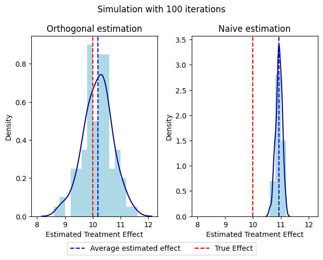
Next we run the simulations with 100, 1000, and 10000 iterations and plot the histograms for the Naive and Orthogonal estimations
Bs = [100, 1000, 10000]

for B in Bs:
    start_time = time.time()
    Naive, Orthogonal = run_simulation(B)
    end_time = time.time()
    elapsed_time = end_time - start_time  # Calculate elapsed time

    fig, axs = plt.subplots(1, 2, sharex=True, tight_layout=True)
    axs[0].hist(Orthogonal, range=(8,12), density=True, bins=Orto_breaks, color='lightblue')
    axs[1].hist(Naive, range=(8,12), density=True, bins=Naive_breaks, color='lightblue')
    sns.kdeplot(Orthogonal, ax=axs[0], color='darkblue')
    sns.kdeplot(Naive, ax=axs[1], color='darkblue')

    axs[0].axvline(x=np.mean(Orthogonal), color='blue', linestyle='--', label='Average estimated effect')
    axs[1].axvline(x=np.mean(Naive), color='blue', linestyle='--', label='Average estimated effect')
    axs[0].axvline(x=10, color='red', linestyle='--', label='True Effect')
    axs[1].axvline(x=10, color='red', linestyle='--', label='True Effect')
    axs[0].title.set_text('Orthogonal estimation')
    axs[1].title.set_text('Naive estimation')
    axs[0].set_xlabel('Estimated Treatment Effect')
    axs[1].set_xlabel('Estimated Treatment Effect')
    handles, labels = axs[0].get_legend_handles_labels()
    fig.legend(handles, labels, loc='lower center', ncol=3, bbox_to_anchor=(0.5, -0.05))
    plt.suptitle(f'Simulation with {B} iterations')
    plt.show()

    print(f'Time taken for {B} iteration simulation: {elapsed_time:.2f} seconds')
Time taken for 100 iteration simulation: 8.57 seconds
Exception in thread Thread-8 (_handle_workers):
Traceback (most recent call last):
  File "C:\Users\Matias Villalba\AppData\Local\Programs\Python\Python312\Lib\threading.py", line 1073, in _bootstrap_inner
    self.run()
  File "C:\Users\Matias Villalba\AppData\Roaming\Python\Python312\site-packages\ipykernel\ipkernel.py", line 761, in run_closure
    _threading_Thread_run(self)
  File "C:\Users\Matias Villalba\AppData\Local\Programs\Python\Python312\Lib\threading.py", line 1010, in run
    self._target(*self._args, **self._kwargs)
  File "C:\Users\Matias Villalba\AppData\Local\Programs\Python\Python312\Lib\site-packages\multiprocess\pool.py", line 516, in _handle_workers
    cls._maintain_pool(ctx, Process, processes, pool, inqueue,
  File "C:\Users\Matias Villalba\AppData\Local\Programs\Python\Python312\Lib\site-packages\multiprocess\pool.py", line 340, in _maintain_pool
    Pool._repopulate_pool_static(ctx, Process, processes, pool,
  File "C:\Users\Matias Villalba\AppData\Local\Programs\Python\Python312\Lib\site-packages\multiprocess\pool.py", line 329, in _repopulate_pool_static
    w.start()
  File "C:\Users\Matias Villalba\AppData\Local\Programs\Python\Python312\Lib\site-packages\multiprocess\process.py", line 121, in start
    self._popen = self._Popen(self)
                  ^^^^^^^^^^^^^^^^^
  File "C:\Users\Matias Villalba\AppData\Local\Programs\Python\Python312\Lib\site-packages\multiprocess\context.py", line 337, in _Popen
    return Popen(process_obj)
           ^^^^^^^^^^^^^^^^^^
  File "C:\Users\Matias Villalba\AppData\Local\Programs\Python\Python312\Lib\site-packages\multiprocess\popen_spawn_win32.py", line 95, in __init__
    reduction.dump(process_obj, to_child)
  File "C:\Users\Matias Villalba\AppData\Local\Programs\Python\Python312\Lib\site-packages\multiprocess\reduction.py", line 63, in dump
    ForkingPickler(file, protocol, *args, **kwds).dump(obj)
  File "C:\Users\Matias Villalba\AppData\Local\Programs\Python\Python312\Lib\site-packages\dill\_dill.py", line 420, in dump
    StockPickler.dump(self, obj)
  File "C:\Users\Matias Villalba\AppData\Local\Programs\Python\Python312\Lib\pickle.py", line 481, in dump
    self.save(obj)
  File "C:\Users\Matias Villalba\AppData\Local\Programs\Python\Python312\Lib\site-packages\dill\_dill.py", line 414, in save
    StockPickler.save(self, obj, save_persistent_id)
  File "C:\Users\Matias Villalba\AppData\Local\Programs\Python\Python312\Lib\pickle.py", line 597, in save
    self.save_reduce(obj=obj, *rv)
  File "C:\Users\Matias Villalba\AppData\Local\Programs\Python\Python312\Lib\pickle.py", line 711, in save_reduce
    save(state)
  File "C:\Users\Matias Villalba\AppData\Local\Programs\Python\Python312\Lib\site-packages\dill\_dill.py", line 414, in save
    StockPickler.save(self, obj, save_persistent_id)
  File "C:\Users\Matias Villalba\AppData\Local\Programs\Python\Python312\Lib\pickle.py", line 554, in save
    f(self, obj)  # Call unbound method with explicit self
    ^^^^^^^^^^^^
  File "C:\Users\Matias Villalba\AppData\Local\Programs\Python\Python312\Lib\site-packages\dill\_dill.py", line 1217, in save_module_dict
    StockPickler.save_dict(pickler, obj)
  File "C:\Users\Matias Villalba\AppData\Local\Programs\Python\Python312\Lib\pickle.py", line 966, in save_dict
    self._batch_setitems(obj.items())
  File "C:\Users\Matias Villalba\AppData\Local\Programs\Python\Python312\Lib\pickle.py", line 990, in _batch_setitems
    save(v)
  File "C:\Users\Matias Villalba\AppData\Local\Programs\Python\Python312\Lib\site-packages\dill\_dill.py", line 414, in save
    StockPickler.save(self, obj, save_persistent_id)
  File "C:\Users\Matias Villalba\AppData\Local\Programs\Python\Python312\Lib\pickle.py", line 554, in save
    f(self, obj)  # Call unbound method with explicit self
    ^^^^^^^^^^^^
  File "C:\Users\Matias Villalba\AppData\Local\Programs\Python\Python312\Lib\pickle.py", line 896, in save_tuple
    save(element)
  File "C:\Users\Matias Villalba\AppData\Local\Programs\Python\Python312\Lib\site-packages\dill\_dill.py", line 414, in save
    StockPickler.save(self, obj, save_persistent_id)
  File "C:\Users\Matias Villalba\AppData\Local\Programs\Python\Python312\Lib\pickle.py", line 597, in save
    self.save_reduce(obj=obj, *rv)
  File "C:\Users\Matias Villalba\AppData\Local\Programs\Python\Python312\Lib\pickle.py", line 711, in save_reduce
    save(state)
  File "C:\Users\Matias Villalba\AppData\Local\Programs\Python\Python312\Lib\site-packages\dill\_dill.py", line 414, in save
    StockPickler.save(self, obj, save_persistent_id)
  File "C:\Users\Matias Villalba\AppData\Local\Programs\Python\Python312\Lib\pickle.py", line 554, in save
    f(self, obj)  # Call unbound method with explicit self
    ^^^^^^^^^^^^
  File "C:\Users\Matias Villalba\AppData\Local\Programs\Python\Python312\Lib\pickle.py", line 896, in save_tuple
    save(element)
  File "C:\Users\Matias Villalba\AppData\Local\Programs\Python\Python312\Lib\site-packages\dill\_dill.py", line 414, in save
    StockPickler.save(self, obj, save_persistent_id)
  File "C:\Users\Matias Villalba\AppData\Local\Programs\Python\Python312\Lib\pickle.py", line 572, in save
    rv = reduce(self.proto)
         ^^^^^^^^^^^^^^^^^^
  File "C:\Users\Matias Villalba\AppData\Local\Programs\Python\Python312\Lib\site-packages\multiprocess\synchronize.py", line 110, in __getstate__
    h = context.get_spawning_popen().duplicate_for_child(sl.handle)
        ^^^^^^^^^^^^^^^^^^^^^^^^^^^^^^^^^^^^^^^^^^^^^^^^^^^^^^^^^^^
  File "C:\Users\Matias Villalba\AppData\Local\Programs\Python\Python312\Lib\site-packages\multiprocess\popen_spawn_win32.py", line 101, in duplicate_for_child
    return reduction.duplicate(handle, self.sentinel)
           ^^^^^^^^^^^^^^^^^^^^^^^^^^^^^^^^^^^^^^^^^^
  File "C:\Users\Matias Villalba\AppData\Local\Programs\Python\Python312\Lib\site-packages\multiprocess\reduction.py", line 82, in duplicate
    return _winapi.DuplicateHandle(
           ^^^^^^^^^^^^^^^^^^^^^^^^
PermissionError: [WinError 5] Access is denied
We can se that the orthogonal estimation yields on average a coeficient more centered on the true effect than the naive estimation. This method of estimation that utilizes the residuals of lasso regresion and helps reduce bias more efficiently than the naive estimation method. This is because it leverages the properties explained on the begining of this notebook rather than just controlling for a relevant set of covariates which may induce endogeneity.
We have used parallel computing because it is supposed to allow us to achieve better processing times. It can significantly lower the running time of computations due to its ability to distribute the workload across multiple processing units.
As an example, we can see how long it would have taken to run the simulation with 1000 iteration if we had not utilized parallel computing.
Without parallel computing
np.random.seed(0)
B = 1000
Naive = np.zeros( B )
Orthogonal = np.zeros( B )

start_time = time.time()
for i in range( 0, B ):
    n = 100
    p = 100
    beta = ( 1 / (np.arange( 1, p + 1 ) ** 2 ) ).reshape( p , 1 )
    gamma = ( 1 / (np.arange( 1, p + 1 ) ** 2 ) ).reshape( p , 1 )

    mean = 0
    sd = 1
    X = np.random.normal( mean , sd, n * p ).reshape( n, p )

    D = ( X @ gamma ) + np.random.normal( mean , sd, n ).reshape( n, 1 )/4 # We reshape because in r when we sum a vecto with a matrix it sum by column

    # DGP
    Y = 10*D + ( X @ beta ) + np.random.normal( mean , sd, n ).reshape( n, 1 )

    # single selection method
    r_lasso_estimation = hdmpy.rlasso( np.concatenate( ( D , X ) , axis  =  1 ) , Y , post = True ) # Regress main equation by lasso

    coef_array = r_lasso_estimation.est[ 'coefficients' ].iloc[ 2:, :].to_numpy()    # Get "X" coefficients

    SX_IDs = np.where( coef_array != 0 )[0]

    # In case all X coefficients are zero, then regress Y on D
    if sum(SX_IDs) == 0 :
        Naive[ i ] = sm.OLS( Y , sm.add_constant(D) ).fit().summary2().tables[1].round(3).iloc[ 1, 0 ]

    # Otherwise, then regress Y on X and D (but only in the selected coefficients)
    elif sum( SX_IDs ) > 0 :
        X_D = np.concatenate( ( D, X[:, SX_IDs ] ) , axis = 1 )
        Naive[ i ] = sm.OLS( Y , sm.add_constant( X_D ) ).fit().summary2().tables[1].round(3).iloc[ 1, 0]

    # In both cases we save D coefficient

    # Regress residuals.
    resY = hdmpy.rlasso( X , Y , post = False ).est[ 'residuals' ]
    resD = hdmpy.rlasso( X , D , post = False ).est[ 'residuals' ]
    Orthogonal[ i ] = sm.OLS( resY , sm.add_constant( resD ) ).fit().summary2().tables[1].round(3).iloc[ 1, 0]
end_time = time.time()
elapsed_time = end_time - start_time  # Calculate elapsed time
print(f'Time taken for {B} iteration simulation without multiprocessing: {elapsed_time:.2f} seconds')
Time taken for 1000 iteration simulation without multiprocessing: 488.92 seconds
We can see that if we were to not use parallel computing, the processing time would be higher. It took 488 seconds to achieve what we achieved in 79.
2.2. Double Lasso - Using School data#
# Libraries
import numpy as np
import pandas as pd
import matplotlib.pyplot as plt
import statsmodels.api as sm
import statsmodels.formula.api as smf
from stargazer.stargazer import Stargazer
from sklearn.model_selection import train_test_split
from sklearn.preprocessing import StandardScaler
from sklearn.linear_model import LassoCV
2.2.1. Preprocessing data#
# Read csv file
df = pd.read_csv('./data/bruhn2016.csv', delimiter=',')
df.head()
| outcome.test.score | treatment | school | is.female | mother.attended.secondary.school | father.attened.secondary.school | failed.at.least.one.school.year | family.receives.cash.transfer | has.computer.with.internet.at.home | is.unemployed | has.some.form.of.income | saves.money.for.future.purchases | intention.to.save.index | makes.list.of.expenses.every.month | negotiates.prices.or.payment.methods | financial.autonomy.index | |
|---|---|---|---|---|---|---|---|---|---|---|---|---|---|---|---|---|
| 0 | 47.367374 | 0 | 17018390 | NaN | NaN | NaN | NaN | NaN | NaN | 1.0 | 1.0 | 0.0 | 29.0 | 0.0 | 1.0 | 52.0 |
| 1 | 58.176758 | 1 | 33002614 | NaN | NaN | NaN | NaN | NaN | NaN | 0.0 | 0.0 | 0.0 | 41.0 | 0.0 | 0.0 | 27.0 |
| 2 | 56.671661 | 1 | 35002914 | 1.0 | 1.0 | 1.0 | 0.0 | 0.0 | 0.0 | 1.0 | 0.0 | 0.0 | 48.0 | 0.0 | 1.0 | 56.0 |
| 3 | 29.079376 | 0 | 35908915 | 1.0 | 0.0 | 0.0 | 0.0 | 0.0 | 0.0 | 0.0 | 0.0 | 0.0 | 42.0 | 0.0 | 0.0 | 27.0 |
| 4 | 49.563534 | 1 | 33047324 | 1.0 | 0.0 | 0.0 | 0.0 | 0.0 | 1.0 | 0.0 | 1.0 | 0.0 | 50.0 | 0.0 | 1.0 | 31.0 |
# Drop missing values, we lose 5077 values (from 17299 to 12222 rows)
df.dropna(axis=0, inplace=True)
df.reset_index(inplace=True ,drop=True)
df.columns
Index(['outcome.test.score', 'treatment', 'school', 'is.female',
       'mother.attended.secondary.school', 'father.attened.secondary.school',
       'failed.at.least.one.school.year', 'family.receives.cash.transfer',
       'has.computer.with.internet.at.home', 'is.unemployed',
       'has.some.form.of.income', 'saves.money.for.future.purchases',
       'intention.to.save.index', 'makes.list.of.expenses.every.month',
       'negotiates.prices.or.payment.methods', 'financial.autonomy.index'],
      dtype='object')
dependent_vars = ['outcome.test.score', 'intention.to.save.index', 'negotiates.prices.or.payment.methods', 'has.some.form.of.income', 'makes.list.of.expenses.every.month', 'financial.autonomy.index', 'saves.money.for.future.purchases', 'is.unemployed']
For Lasso regressions, we split the data into train and test data, and standarize the covariates matrix
# Train test split
X = df.drop(dependent_vars, axis = 1)
y = df[dependent_vars]

X_train, X_test, y_train, y_test = train_test_split(X, y, test_size = 0.2, random_state = 42)
T_train = X_train['treatment']
T_test = X_test['treatment']

X_train = X_train.drop(['treatment'], axis = 1)
X_test = X_test.drop(['treatment'], axis = 1)
# Standarize X data
scale = StandardScaler()

X_train_scaled = pd.DataFrame(scale.fit_transform(X_train), index=X_train.index)
X_test_scaled = pd.DataFrame(scale.transform(X_test), index=X_test.index)
X_scaled = pd.concat([X_train_scaled, X_test_scaled]).sort_index()
T = pd.concat([T_train, T_test]).sort_index()
2.2.2. Regressions#
a. OLS#
From 1 - 3 regression: measures treatment impact on student financial proficiency
From 4 - 6 regression: measures treatment impact on student savings behavior and attitudes
From 7 - 9 regression: measures treatment impact on student money management behavior and attitudes
From 10 - 12 regression: measures treatment impact on student entrepreneurship and work outcomes
# Rgeressions with "Student Financial Proficiency" as dependet variable
ols_score_1      = sm.OLS.from_formula('Q("outcome.test.score") ~ treatment', data=df).fit()
ols_score_2      = sm.OLS.from_formula('Q("outcome.test.score") ~ treatment + school + Q("failed.at.least.one.school.year")', data=df).fit()
ols_score_3      = sm.OLS.from_formula('Q("outcome.test.score") ~ treatment + school + Q("failed.at.least.one.school.year") + Q("is.female") + Q("mother.attended.secondary.school") + Q("father.attened.secondary.school") + Q("family.receives.cash.transfer") + Q("has.computer.with.internet.at.home")', data=df).fit()

# Rgeressions with "Intention to save index" as dependet variable
ols_saving_1     = sm.OLS.from_formula('Q("intention.to.save.index") ~ treatment', data=df).fit()
ols_saving_2     = sm.OLS.from_formula('Q("intention.to.save.index") ~ treatment + school + Q("failed.at.least.one.school.year")', data=df).fit()
ols_saving_3     = sm.OLS.from_formula('Q("intention.to.save.index") ~ treatment + school + Q("failed.at.least.one.school.year") + Q("is.female") + Q("mother.attended.secondary.school") + Q("father.attened.secondary.school") + Q("family.receives.cash.transfer") + Q("has.computer.with.internet.at.home")', data=df).fit()

# Rgeressions with "Negotiates prices or payment methods" as dependet variable
ols_negotiates_1 = sm.OLS.from_formula('Q("negotiates.prices.or.payment.methods") ~ treatment', data=df).fit()
ols_negotiates_2 = sm.OLS.from_formula('Q("negotiates.prices.or.payment.methods") ~ treatment + school + Q("failed.at.least.one.school.year")', data=df).fit()
ols_negotiates_3 = sm.OLS.from_formula('Q("negotiates.prices.or.payment.methods") ~ treatment + school + Q("failed.at.least.one.school.year") + Q("is.female") + Q("mother.attended.secondary.school") + Q("father.attened.secondary.school") + Q("family.receives.cash.transfer") + Q("has.computer.with.internet.at.home")', data=df).fit()

# Rgeressions with "Has some form of income" as dependet variable
ols_manage_1     = sm.OLS.from_formula('Q("has.some.form.of.income") ~ treatment', data=df).fit()
ols_manage_2     = sm.OLS.from_formula('Q("has.some.form.of.income") ~ treatment + school + Q("failed.at.least.one.school.year")', data=df).fit()
ols_manage_3     = sm.OLS.from_formula('Q("has.some.form.of.income") ~ treatment + school + Q("failed.at.least.one.school.year") + Q("is.female") + Q("mother.attended.secondary.school") + Q("father.attened.secondary.school") + Q("family.receives.cash.transfer") + Q("has.computer.with.internet.at.home")', data=df).fit()

# Show parameters in table
st = Stargazer([ols_score_1, ols_score_2, ols_score_3, ols_saving_1, ols_saving_2, ols_saving_3, ols_negotiates_1, ols_negotiates_2, ols_negotiates_3, ols_manage_1, ols_manage_2, ols_manage_3])
st.custom_columns(["Dependent var 1: Student Financial Proficiency", "Dependent var 2: Intention to save index", "Dependent var 3: Negotiates prices or payment methods", "Dependent var 4: Has some form of income"], [3, 3, 3, 3])
st.rename_covariates({'Q("failed.at.least.one.school.year")': 'Failed at least one school year', 'Q("is.female")': 'Female', 'Q("father.attened.secondary.school")': 'Father attended secondary school', 'Q("Family.receives.cash.transfer")': 'Family receives cash transfer', 'Q("has.computer.with.internet.at.home")': 'Has computer with internet at home'})
st
Intel MKL WARNING: Support of Intel(R) Streaming SIMD Extensions 4.2 (Intel(R) SSE4.2) enabled only processors has been deprecated. Intel oneAPI Math Kernel Library 2025.0 will require Intel(R) Advanced Vector Extensions (Intel(R) AVX) instructions.
Intel MKL WARNING: Support of Intel(R) Streaming SIMD Extensions 4.2 (Intel(R) SSE4.2) enabled only processors has been deprecated. Intel oneAPI Math Kernel Library 2025.0 will require Intel(R) Advanced Vector Extensions (Intel(R) AVX) instructions.
Intel MKL WARNING: Support of Intel(R) Streaming SIMD Extensions 4.2 (Intel(R) SSE4.2) enabled only processors has been deprecated. Intel oneAPI Math Kernel Library 2025.0 will require Intel(R) Advanced Vector Extensions (Intel(R) AVX) instructions.
Intel MKL WARNING: Support of Intel(R) Streaming SIMD Extensions 4.2 (Intel(R) SSE4.2) enabled only processors has been deprecated. Intel oneAPI Math Kernel Library 2025.0 will require Intel(R) Advanced Vector Extensions (Intel(R) AVX) instructions.
Intel MKL WARNING: Support of Intel(R) Streaming SIMD Extensions 4.2 (Intel(R) SSE4.2) enabled only processors has been deprecated. Intel oneAPI Math Kernel Library 2025.0 will require Intel(R) Advanced Vector Extensions (Intel(R) AVX) instructions.
Intel MKL WARNING: Support of Intel(R) Streaming SIMD Extensions 4.2 (Intel(R) SSE4.2) enabled only processors has been deprecated. Intel oneAPI Math Kernel Library 2025.0 will require Intel(R) Advanced Vector Extensions (Intel(R) AVX) instructions.
Intel MKL WARNING: Support of Intel(R) Streaming SIMD Extensions 4.2 (Intel(R) SSE4.2) enabled only processors has been deprecated. Intel oneAPI Math Kernel Library 2025.0 will require Intel(R) Advanced Vector Extensions (Intel(R) AVX) instructions.
Intel MKL WARNING: Support of Intel(R) Streaming SIMD Extensions 4.2 (Intel(R) SSE4.2) enabled only processors has been deprecated. Intel oneAPI Math Kernel Library 2025.0 will require Intel(R) Advanced Vector Extensions (Intel(R) AVX) instructions.
Intel MKL WARNING: Support of Intel(R) Streaming SIMD Extensions 4.2 (Intel(R) SSE4.2) enabled only processors has been deprecated. Intel oneAPI Math Kernel Library 2025.0 will require Intel(R) Advanced Vector Extensions (Intel(R) AVX) instructions.
Intel MKL WARNING: Support of Intel(R) Streaming SIMD Extensions 4.2 (Intel(R) SSE4.2) enabled only processors has been deprecated. Intel oneAPI Math Kernel Library 2025.0 will require Intel(R) Advanced Vector Extensions (Intel(R) AVX) instructions.
Intel MKL WARNING: Support of Intel(R) Streaming SIMD Extensions 4.2 (Intel(R) SSE4.2) enabled only processors has been deprecated. Intel oneAPI Math Kernel Library 2025.0 will require Intel(R) Advanced Vector Extensions (Intel(R) AVX) instructions.
Intel MKL WARNING: Support of Intel(R) Streaming SIMD Extensions 4.2 (Intel(R) SSE4.2) enabled only processors has been deprecated. Intel oneAPI Math Kernel Library 2025.0 will require Intel(R) Advanced Vector Extensions (Intel(R) AVX) instructions.
| Dependent var 1: Student Financial Proficiency | Dependent var 2: Intention to save index | Dependent var 3: Negotiates prices or payment methods | Dependent var 4: Has some form of income | |||||||||
| (1) | (2) | (3) | (4) | (5) | (6) | (7) | (8) | (9) | (10) | (11) | (12) | |
| Intercept | 57.591*** | 59.377*** | 58.860*** | 49.016*** | 46.725*** | 46.603*** | 0.763*** | 0.856*** | 0.855*** | 0.639*** | 0.534*** | 0.609*** |
| (0.187) | (0.556) | (0.675) | (0.240) | (0.728) | (0.890) | (0.006) | (0.017) | (0.020) | (0.006) | (0.019) | (0.023) | |
| Failed at least one school year | -7.218*** | -6.652*** | -3.614*** | -3.315*** | 0.024*** | 0.013 | 0.005 | 0.006 | ||||
| (0.288) | (0.289) | (0.377) | (0.381) | (0.009) | (0.009) | (0.010) | (0.010) | |||||
| Q("family.receives.cash.transfer") | -1.837*** | -1.189*** | 0.028*** | -0.027*** | ||||||||
| (0.283) | (0.374) | (0.009) | (0.010) | |||||||||
| Father attended secondary school | 0.875*** | -0.213 | -0.012 | 0.021** | ||||||||
| (0.298) | (0.392) | (0.009) | (0.010) | |||||||||
| Has computer with internet at home | -0.505* | -0.276 | 0.024*** | -0.035*** | ||||||||
| (0.281) | (0.371) | (0.009) | (0.010) | |||||||||
| Female | 2.943*** | 1.403*** | -0.069*** | -0.051*** | ||||||||
| (0.257) | (0.339) | (0.008) | (0.009) | |||||||||
| Q("mother.attended.secondary.school") | 0.968*** | 1.192*** | 0.001 | 0.013 | ||||||||
| (0.295) | (0.388) | (0.009) | (0.010) | |||||||||
| school | 0.000 | -0.000** | 0.000*** | 0.000*** | -0.000*** | -0.000*** | 0.000*** | 0.000*** | ||||
| (0.000) | (0.000) | (0.000) | (0.000) | (0.000) | (0.000) | (0.000) | (0.000) | |||||
| treatment | 4.216*** | 4.392*** | 4.325*** | -0.070 | -0.005 | -0.032 | 0.001 | 0.001 | 0.003 | 0.017** | 0.016* | 0.018** |
| (0.261) | (0.255) | (0.253) | (0.335) | (0.334) | (0.333) | (0.008) | (0.008) | (0.008) | (0.009) | (0.009) | (0.009) | |
| Observations | 12222 | 12222 | 12222 | 12222 | 12222 | 12222 | 12222 | 12222 | 12222 | 12222 | 12222 | 12222 |
| R2 | 0.021 | 0.069 | 0.086 | 0.000 | 0.009 | 0.013 | 0.000 | 0.004 | 0.012 | 0.000 | 0.003 | 0.011 |
| Adjusted R2 | 0.021 | 0.068 | 0.085 | -0.000 | 0.009 | 0.012 | -0.000 | 0.004 | 0.012 | 0.000 | 0.003 | 0.010 |
| Residual Std. Error | 14.432 (df=12220) | 14.076 (df=12218) | 13.949 (df=12213) | 18.506 (df=12220) | 18.421 (df=12218) | 18.393 (df=12213) | 0.425 (df=12220) | 0.424 (df=12218) | 0.423 (df=12213) | 0.478 (df=12220) | 0.477 (df=12218) | 0.475 (df=12213) |
| F Statistic | 260.547*** (df=1; 12220) | 300.463*** (df=3; 12218) | 143.315*** (df=8; 12213) | 0.043 (df=1; 12220) | 38.533*** (df=3; 12218) | 19.812*** (df=8; 12213) | 0.018 (df=1; 12220) | 16.352*** (df=3; 12218) | 18.841*** (df=8; 12213) | 3.843** (df=1; 12220) | 12.839*** (df=3; 12218) | 16.603*** (df=8; 12213) |
| Note: | *p<0.1; **p<0.05; ***p<0.01 | |||||||||||
# Save the ITT beta and the confidence intervals
beta_OLS = ols_score_3.params['treatment']
conf_int_OLS = ols_score_3.conf_int().loc['treatment']
b. Double Lasso using cross validation#
We use the first dependent variable (Student Financial Proficiency)
Step 1: We ran Lasso regression of Y (student financial proficiency) on X, and T (treatment) on X
lasso_CV_yX = LassoCV(alphas = np.arange(0.0001, 0.5, 0.001), cv = 10, max_iter = 5000)
lasso_CV_yX.fit(X_train_scaled, y_train['outcome.test.score'])

lasso_CV_lambda = lasso_CV_yX.alpha_
print(f"Mejor lambda: {lasso_CV_lambda:.4f}")
Intel MKL WARNING: Support of Intel(R) Streaming SIMD Extensions 4.2 (Intel(R) SSE4.2) enabled only processors has been deprecated. Intel oneAPI Math Kernel Library 2025.0 will require Intel(R) Advanced Vector Extensions (Intel(R) AVX) instructions.
Intel MKL WARNING: Support of Intel(R) Streaming SIMD Extensions 4.2 (Intel(R) SSE4.2) enabled only processors has been deprecated. Intel oneAPI Math Kernel Library 2025.0 will require Intel(R) Advanced Vector Extensions (Intel(R) AVX) instructions.
Intel MKL WARNING: Support of Intel(R) Streaming SIMD Extensions 4.2 (Intel(R) SSE4.2) enabled only processors has been deprecated. Intel oneAPI Math Kernel Library 2025.0 will require Intel(R) Advanced Vector Extensions (Intel(R) AVX) instructions.
Intel MKL WARNING: Support of Intel(R) Streaming SIMD Extensions 4.2 (Intel(R) SSE4.2) enabled only processors has been deprecated. Intel oneAPI Math Kernel Library 2025.0 will require Intel(R) Advanced Vector Extensions (Intel(R) AVX) instructions.
Intel MKL WARNING: Support of Intel(R) Streaming SIMD Extensions 4.2 (Intel(R) SSE4.2) enabled only processors has been deprecated. Intel oneAPI Math Kernel Library 2025.0 will require Intel(R) Advanced Vector Extensions (Intel(R) AVX) instructions.
Intel MKL WARNING: Support of Intel(R) Streaming SIMD Extensions 4.2 (Intel(R) SSE4.2) enabled only processors has been deprecated. Intel oneAPI Math Kernel Library 2025.0 will require Intel(R) Advanced Vector Extensions (Intel(R) AVX) instructions.
Intel MKL WARNING: Support of Intel(R) Streaming SIMD Extensions 4.2 (Intel(R) SSE4.2) enabled only processors has been deprecated. Intel oneAPI Math Kernel Library 2025.0 will require Intel(R) Advanced Vector Extensions (Intel(R) AVX) instructions.
Intel MKL WARNING: Support of Intel(R) Streaming SIMD Extensions 4.2 (Intel(R) SSE4.2) enabled only processors has been deprecated. Intel oneAPI Math Kernel Library 2025.0 will require Intel(R) Advanced Vector Extensions (Intel(R) AVX) instructions.
Intel MKL WARNING: Support of Intel(R) Streaming SIMD Extensions 4.2 (Intel(R) SSE4.2) enabled only processors has been deprecated. Intel oneAPI Math Kernel Library 2025.0 will require Intel(R) Advanced Vector Extensions (Intel(R) AVX) instructions.
Intel MKL WARNING: Support of Intel(R) Streaming SIMD Extensions 4.2 (Intel(R) SSE4.2) enabled only processors has been deprecated. Intel oneAPI Math Kernel Library 2025.0 will require Intel(R) Advanced Vector Extensions (Intel(R) AVX) instructions.
Mejor lambda: 0.0001
# Estimate y predictions with all X
y_pred_yX = lasso_CV_yX.predict(X_scaled)
lasso_CV_TX = LassoCV(alphas = np.arange(0.0001, 0.5, 0.001), cv = 10, max_iter = 5000)
lasso_CV_TX.fit(X_train_scaled, T_train)
y_pred = lasso_CV_TX.predict(X_test_scaled)

lasso_CV_lambda = lasso_CV_TX.alpha_
print(f"Mejor lambda: {lasso_CV_lambda:.4f}")
Intel MKL WARNING: Support of Intel(R) Streaming SIMD Extensions 4.2 (Intel(R) SSE4.2) enabled only processors has been deprecated. Intel oneAPI Math Kernel Library 2025.0 will require Intel(R) Advanced Vector Extensions (Intel(R) AVX) instructions.
Intel MKL WARNING: Support of Intel(R) Streaming SIMD Extensions 4.2 (Intel(R) SSE4.2) enabled only processors has been deprecated. Intel oneAPI Math Kernel Library 2025.0 will require Intel(R) Advanced Vector Extensions (Intel(R) AVX) instructions.
Intel MKL WARNING: Support of Intel(R) Streaming SIMD Extensions 4.2 (Intel(R) SSE4.2) enabled only processors has been deprecated. Intel oneAPI Math Kernel Library 2025.0 will require Intel(R) Advanced Vector Extensions (Intel(R) AVX) instructions.
Intel MKL WARNING: Support of Intel(R) Streaming SIMD Extensions 4.2 (Intel(R) SSE4.2) enabled only processors has been deprecated. Intel oneAPI Math Kernel Library 2025.0 will require Intel(R) Advanced Vector Extensions (Intel(R) AVX) instructions.
Intel MKL WARNING: Support of Intel(R) Streaming SIMD Extensions 4.2 (Intel(R) SSE4.2) enabled only processors has been deprecated. Intel oneAPI Math Kernel Library 2025.0 will require Intel(R) Advanced Vector Extensions (Intel(R) AVX) instructions.
Intel MKL WARNING: Support of Intel(R) Streaming SIMD Extensions 4.2 (Intel(R) SSE4.2) enabled only processors has been deprecated. Intel oneAPI Math Kernel Library 2025.0 will require Intel(R) Advanced Vector Extensions (Intel(R) AVX) instructions.
Intel MKL WARNING: Support of Intel(R) Streaming SIMD Extensions 4.2 (Intel(R) SSE4.2) enabled only processors has been deprecated. Intel oneAPI Math Kernel Library 2025.0 will require Intel(R) Advanced Vector Extensions (Intel(R) AVX) instructions.
Intel MKL WARNING: Support of Intel(R) Streaming SIMD Extensions 4.2 (Intel(R) SSE4.2) enabled only processors has been deprecated. Intel oneAPI Math Kernel Library 2025.0 will require Intel(R) Advanced Vector Extensions (Intel(R) AVX) instructions.
Intel MKL WARNING: Support of Intel(R) Streaming SIMD Extensions 4.2 (Intel(R) SSE4.2) enabled only processors has been deprecated. Intel oneAPI Math Kernel Library 2025.0 will require Intel(R) Advanced Vector Extensions (Intel(R) AVX) instructions.
Intel MKL WARNING: Support of Intel(R) Streaming SIMD Extensions 4.2 (Intel(R) SSE4.2) enabled only processors has been deprecated. Intel oneAPI Math Kernel Library 2025.0 will require Intel(R) Advanced Vector Extensions (Intel(R) AVX) instructions.
Mejor lambda: 0.0011
# Estimate T predictions with all X
y_pred_TX = lasso_CV_TX.predict(X_scaled)
Step 2: Obtain the resulting residuals
res_yX = y['outcome.test.score'] - y_pred_yX
res_TX = T - y_pred_TX
Step 3: We run the least squares of res_yX on res_TX
ols_score_b = sm.OLS.from_formula('res_yX ~ res_TX', data=df).fit()

# Show parameters in table
st = Stargazer([ols_score_b])
st
Intel MKL WARNING: Support of Intel(R) Streaming SIMD Extensions 4.2 (Intel(R) SSE4.2) enabled only processors has been deprecated. Intel oneAPI Math Kernel Library 2025.0 will require Intel(R) Advanced Vector Extensions (Intel(R) AVX) instructions.
| Dependent variable: res_yX | |
| (1) | |
| Intercept | 0.033 |
| (0.126) | |
| res_TX | 4.324*** |
| (0.253) | |
| Observations | 12222 |
| R2 | 0.023 |
| Adjusted R2 | 0.023 |
| Residual Std. Error | 13.945 (df=12220) |
| F Statistic | 292.956*** (df=1; 12220) |
| Note: | *p<0.1; **p<0.05; ***p<0.01 |
# Save the ITT beta and the confidence intervals
beta_DL_CV = ols_score_b.params['res_TX']
conf_int_DL_CV = ols_score_b.conf_int().loc['res_TX']
c. Double Lasso using theoretical lambda#
# !pip install multiprocess
# !pip install pyreadr
# !git clone https://github.com/maxhuppertz/hdmpy.git
import sys
sys.path.insert(1, "./hdmpy")
# We wrap the package so that it has the familiar sklearn API
import hdmpy
from sklearn.base import BaseEstimator, clone

class RLasso(BaseEstimator):

    def __init__(self, *, post=True):
        self.post = post

    def fit(self, X, y):
        self.rlasso_ = hdmpy.rlasso(X, y, post=self.post)
        return self

    def predict(self, X):
        return np.array(X) @ np.array(self.rlasso_.est['beta']).flatten() + np.array(self.rlasso_.est['intercept'])

    def nsel(self):
        return sum(abs(np.array(self.rlasso_.est['beta']).flatten()>0))

lasso_model = lambda: RLasso(post=False)
Step 1:
# Estimate y predictions with all X
y_pred_yX = lasso_model().fit(X_scaled, y['outcome.test.score']).predict(X_scaled)
Intel MKL WARNING: Support of Intel(R) Streaming SIMD Extensions 4.2 (Intel(R) SSE4.2) enabled only processors has been deprecated. Intel oneAPI Math Kernel Library 2025.0 will require Intel(R) Advanced Vector Extensions (Intel(R) AVX) instructions.
Intel MKL WARNING: Support of Intel(R) Streaming SIMD Extensions 4.2 (Intel(R) SSE4.2) enabled only processors has been deprecated. Intel oneAPI Math Kernel Library 2025.0 will require Intel(R) Advanced Vector Extensions (Intel(R) AVX) instructions.
Intel MKL WARNING: Support of Intel(R) Streaming SIMD Extensions 4.2 (Intel(R) SSE4.2) enabled only processors has been deprecated. Intel oneAPI Math Kernel Library 2025.0 will require Intel(R) Advanced Vector Extensions (Intel(R) AVX) instructions.
Intel MKL WARNING: Support of Intel(R) Streaming SIMD Extensions 4.2 (Intel(R) SSE4.2) enabled only processors has been deprecated. Intel oneAPI Math Kernel Library 2025.0 will require Intel(R) Advanced Vector Extensions (Intel(R) AVX) instructions.
# Estimate T predictions with all X
y_pred_TX = lasso_model().fit(X_scaled, T).predict(X_scaled)
Intel MKL WARNING: Support of Intel(R) Streaming SIMD Extensions 4.2 (Intel(R) SSE4.2) enabled only processors has been deprecated. Intel oneAPI Math Kernel Library 2025.0 will require Intel(R) Advanced Vector Extensions (Intel(R) AVX) instructions.
Intel MKL WARNING: Support of Intel(R) Streaming SIMD Extensions 4.2 (Intel(R) SSE4.2) enabled only processors has been deprecated. Intel oneAPI Math Kernel Library 2025.0 will require Intel(R) Advanced Vector Extensions (Intel(R) AVX) instructions.
Intel MKL WARNING: Support of Intel(R) Streaming SIMD Extensions 4.2 (Intel(R) SSE4.2) enabled only processors has been deprecated. Intel oneAPI Math Kernel Library 2025.0 will require Intel(R) Advanced Vector Extensions (Intel(R) AVX) instructions.
Intel MKL WARNING: Support of Intel(R) Streaming SIMD Extensions 4.2 (Intel(R) SSE4.2) enabled only processors has been deprecated. Intel oneAPI Math Kernel Library 2025.0 will require Intel(R) Advanced Vector Extensions (Intel(R) AVX) instructions.
Step 2:
res_yX = y['outcome.test.score'] - y_pred_yX
res_TX = T - y_pred_TX
Step 3:
lasso_hdm_score = sm.OLS.from_formula('res_yX ~ res_TX', data=df).fit()

# Show parameters in table
st = Stargazer([lasso_hdm_score])
st
Intel MKL WARNING: Support of Intel(R) Streaming SIMD Extensions 4.2 (Intel(R) SSE4.2) enabled only processors has been deprecated. Intel oneAPI Math Kernel Library 2025.0 will require Intel(R) Advanced Vector Extensions (Intel(R) AVX) instructions.
| Dependent variable: res_yX | |
| (1) | |
| Intercept | 0.000 |
| (0.126) | |
| res_TX | 4.316*** |
| (0.253) | |
| Observations | 12222 |
| R2 | 0.023 |
| Adjusted R2 | 0.023 |
| Residual Std. Error | 13.953 (df=12220) |
| F Statistic | 291.837*** (df=1; 12220) |
| Note: | *p<0.1; **p<0.05; ***p<0.01 |
# Save the ITT beta and the confidence intervals
beta_DL_theo = lasso_hdm_score.params['res_TX']
conf_int_DL_theo = lasso_hdm_score.conf_int().loc['res_TX']
d. Double Lasso using partialling out method#
rlassoEffect = hdmpy.rlassoEffect(X_scaled, y['outcome.test.score'], T, method='partialling out')
Intel MKL WARNING: Support of Intel(R) Streaming SIMD Extensions 4.2 (Intel(R) SSE4.2) enabled only processors has been deprecated. Intel oneAPI Math Kernel Library 2025.0 will require Intel(R) Advanced Vector Extensions (Intel(R) AVX) instructions.
Intel MKL WARNING: Support of Intel(R) Streaming SIMD Extensions 4.2 (Intel(R) SSE4.2) enabled only processors has been deprecated. Intel oneAPI Math Kernel Library 2025.0 will require Intel(R) Advanced Vector Extensions (Intel(R) AVX) instructions.
Intel MKL WARNING: Support of Intel(R) Streaming SIMD Extensions 4.2 (Intel(R) SSE4.2) enabled only processors has been deprecated. Intel oneAPI Math Kernel Library 2025.0 will require Intel(R) Advanced Vector Extensions (Intel(R) AVX) instructions.
Intel MKL WARNING: Support of Intel(R) Streaming SIMD Extensions 4.2 (Intel(R) SSE4.2) enabled only processors has been deprecated. Intel oneAPI Math Kernel Library 2025.0 will require Intel(R) Advanced Vector Extensions (Intel(R) AVX) instructions.
Intel MKL WARNING: Support of Intel(R) Streaming SIMD Extensions 4.2 (Intel(R) SSE4.2) enabled only processors has been deprecated. Intel oneAPI Math Kernel Library 2025.0 will require Intel(R) Advanced Vector Extensions (Intel(R) AVX) instructions.
Intel MKL WARNING: Support of Intel(R) Streaming SIMD Extensions 4.2 (Intel(R) SSE4.2) enabled only processors has been deprecated. Intel oneAPI Math Kernel Library 2025.0 will require Intel(R) Advanced Vector Extensions (Intel(R) AVX) instructions.
Intel MKL WARNING: Support of Intel(R) Streaming SIMD Extensions 4.2 (Intel(R) SSE4.2) enabled only processors has been deprecated. Intel oneAPI Math Kernel Library 2025.0 will require Intel(R) Advanced Vector Extensions (Intel(R) AVX) instructions.
Intel MKL WARNING: Support of Intel(R) Streaming SIMD Extensions 4.2 (Intel(R) SSE4.2) enabled only processors has been deprecated. Intel oneAPI Math Kernel Library 2025.0 will require Intel(R) Advanced Vector Extensions (Intel(R) AVX) instructions.
Intel MKL WARNING: Support of Intel(R) Streaming SIMD Extensions 4.2 (Intel(R) SSE4.2) enabled only processors has been deprecated. Intel oneAPI Math Kernel Library 2025.0 will require Intel(R) Advanced Vector Extensions (Intel(R) AVX) instructions.
Intel MKL WARNING: Support of Intel(R) Streaming SIMD Extensions 4.2 (Intel(R) SSE4.2) enabled only processors has been deprecated. Intel oneAPI Math Kernel Library 2025.0 will require Intel(R) Advanced Vector Extensions (Intel(R) AVX) instructions.
Intel MKL WARNING: Support of Intel(R) Streaming SIMD Extensions 4.2 (Intel(R) SSE4.2) enabled only processors has been deprecated. Intel oneAPI Math Kernel Library 2025.0 will require Intel(R) Advanced Vector Extensions (Intel(R) AVX) instructions.
rlassoEffect
{'alpha': 4.313441,
 'se': array([0.25271166]),
 't': array([17.06862565]),
 'pval': array([2.54111627e-65]),
 'coefficients': 4.313441,
 'coefficient': 4.313441,
 'coefficients_reg':                      0
 (Intercept)  59.769260
 x0            0.000000
 x1            1.511205
 x2            0.529423
 x3            0.461196
 x4           -2.878027
 x5           -0.857569
 x6            0.000000,
 'selection_index': array([[False],
        [ True],
        [ True],
        [ True],
        [ True],
        [ True],
        [False]]),
 'residuals': {'epsilon': array([[-10.04200277],
         [-31.30841071],
         [-15.13769394],
         ...,
         [-17.22383794],
         [ -3.93047339],
         [ -4.88461742]]),
  'v': array([[ 0.48682705],
         [-0.513173  ],
         [ 0.48682705],
         ...,
         [ 0.48682705],
         [-0.513173  ],
         [-0.513173  ]], dtype=float32)},
 'samplesize': 12222}
beta_part_out = rlassoEffect['coefficient']
critical_value = 1.96  # For 95% confidence level

conf_int_part_out = [beta_part_out - critical_value * rlassoEffect['se'], \
                     beta_part_out + critical_value * rlassoEffect['se']]
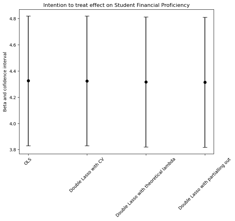
Results#
We found that the intention to treat effect (ITT) is very similar estimating with all 4 models (aproximately 4.3, with 95% of confidence). This could be because the ratio between the parameters and the number of observations p/n is small (8/12222 = 0.00065455735). In other words, we are not dealing with high dimensional data and the models from b. to d. will outperform the OLS when we are in the opposite scenario. In conclusion, we can say that the OLS model estimates the ITT just as good as the other models.
# Plotting the effect size with confidence intervals
plt.figure(figsize=(8, 6))
plt.errorbar('OLS', beta_OLS, yerr=np.array([beta_OLS - conf_int_OLS[0], conf_int_OLS[1] - beta_OLS]).reshape(2, 1),
             fmt='o', color='black', capsize=5)
plt.errorbar('Double Lasso with CV', beta_DL_CV, yerr=np.array([beta_DL_CV - conf_int_DL_CV[0], conf_int_DL_CV[1] - beta_DL_CV]).reshape(2, 1),
             fmt='o', color='black', capsize=5)
plt.errorbar('Double Lasso with theoretical lambda', beta_DL_theo, yerr=np.array([beta_DL_theo - conf_int_DL_theo[0], conf_int_DL_theo[1] - beta_DL_theo]).reshape(2, 1),
             fmt='o', color='black', capsize=5)
plt.errorbar('Double Lasso with partialling out', beta_part_out, yerr=np.array([beta_part_out - conf_int_part_out[0], conf_int_part_out[1] - beta_part_out]).reshape(2, 1),
             fmt='o', color='black', capsize=5)
plt.title('Intention to treat effect on Student Financial Proficiency')
plt.ylabel('Beta and cofidence interval')
plt.xticks(rotation=45)

plt.show()