Lab 4 - R Code#
Authors: Valerie Dube, Erzo Garay, Juan Marcos Guerrero y Matias Villalba
Bootstraping#
install.packages("boot")
Installing package into 'C:/Users/Matias Villalba/AppData/Local/R/win-library/4.3'
(as 'lib' is unspecified)
package 'boot' successfully unpacked and MD5 sums checked
The downloaded binary packages are in
	C:\Users\Matias Villalba\AppData\Local\Temp\Rtmp2ZShEs\downloaded_packages
library(boot)
1. Data base#
The data is not created randomly; it is extracted from the “penn_jae.dat” database. This database is imported and filtered so that the variable “tg” becomes “t4,” which is a dummy variable identifying those treated with t4 versus individuals in the control group.
Penn <- as.data.frame(read.table("../../data/penn_jae.dat", header=T ))
Penn<- subset(Penn, tg==4 | tg==0)
Penn$t4 <- ifelse(Penn$tg == 4, 1, Penn$tg)
Penn$tg <- NULL
attach(Penn)
2. Bootstrap function#
A function is created with the specified linear regression “log(inuidur1)~t4+ (female+black+othrace+factor(dep)+q2+q3+q4+q5+q6+agelt35+agegt54+durable+lusd+husd),” which outputs information about the estimated coefficients.
bootpar.fn <- function(data, index)
  coef(lm(log(inuidur1)~t4+ (female+black+othrace+factor(dep)+q2+q3+q4+q5+q6+agelt35+agegt54+durable+lusd+husd), data = data, subset = index))
reg_lineal = boot(Penn, bootpar.fn, 1000)
3. Standard error#
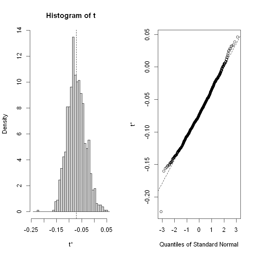
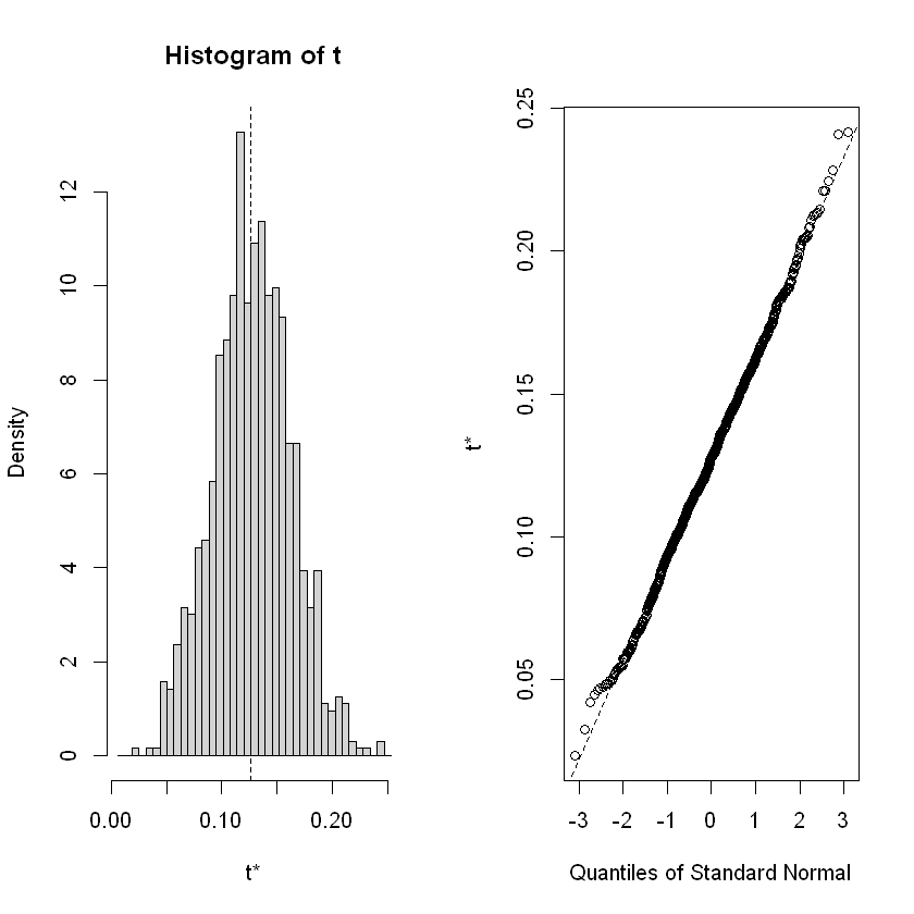
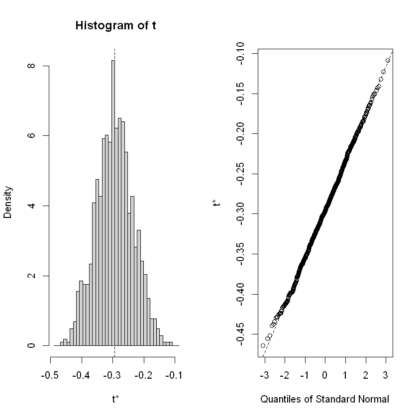
A table is created for the three specified variables: “t4”, “female”, and “black”. Then, the distributions of the estimated parameters for the 1000 iterations are plotted.
original_values <- c(reg_lineal$t0[2], reg_lineal$t0[3], reg_lineal$t0[4])
standard_errors <- c(sd(reg_lineal$t[,2]),sd(reg_lineal$t[,3]), sd(reg_lineal$t[,4]))
table_data <- data.frame(
  "Original" = original_values,
  "Standard Error" = standard_errors
)
print(table_data)
          Original Standard.Error
t4     -0.07169248     0.03589493
female  0.12636833     0.03520114
black  -0.29376798     0.05942533
3.1. t4 distribution#
plot(reg_lineal, index=2)
3.2. Female distribution#
plot(reg_lineal, index=3)
3.3. Black distribution#
plot(reg_lineal, index=4)
Causal Forest#
set.seed(1)
rm(list = ls())
# Installing packages
install.packages("grf")
install.packages("Hmisc")
install.packages("evaluate")
Installing package into 'C:/Users/Matias Villalba/AppData/Local/R/win-library/4.3'
(as 'lib' is unspecified)
library(grf)
if(packageVersion("grf") < '0.10.2') {
  warning("This script requires grf 0.10.2 or higher")
}
library(sandwich)
library(lmtest)
library(Hmisc)
library(ggplot2)
1. Preprocessing#
# Import synthetic data from data folder
data.all = read.csv("../../data/synthetic_data.csv")

data.all$schoolid = factor(data.all$schoolid)
DF = data.all[,-1]
school.id = as.numeric(data.all$schoolid)

school.mat = model.matrix(~ schoolid + 0, data = data.all)
school.size = colSums(school.mat)
# It appears that school ID does not affect pscore. So ignore it
# in modeling, and just treat it as source of per-cluster error.
w.lm = glm(Z ~ ., data = data.all[,-3], family = binomial)
summary(w.lm)

W = DF$Z
Y = DF$Y
X.raw = DF[,-(1:2)]

C1.exp = model.matrix(~ factor(X.raw$C1) + 0)
XC.exp = model.matrix(~ factor(X.raw$XC) + 0)

X = cbind(X.raw[,-which(names(X.raw) %in% c("C1", "XC"))], C1.exp, XC.exp)
Call:
glm(formula = Z ~ ., family = binomial, data = data.all[, -3])

Coefficients: (6 not defined because of singularities)
              Estimate Std. Error z value Pr(>|z|)
(Intercept) -0.9524636  0.2845173  -3.348 0.000815 ***
schoolid2    0.0697302  0.2766287   0.252 0.800986
schoolid3    0.0382080  0.2911323   0.131 0.895586
schoolid4    0.1761334  0.2784711   0.633 0.527059
schoolid5   -0.0033389  0.2950180  -0.011 0.990970
schoolid6    0.0583548  0.3067481   0.190 0.849124
schoolid7   -0.1313759  0.3188190  -0.412 0.680288
schoolid8    0.1233661  0.3023736   0.408 0.683279
schoolid9   -0.1955428  0.3073344  -0.636 0.524611
schoolid10  -0.1892794  0.2968750  -0.638 0.523752
schoolid11  -0.2224060  0.5461005  -0.407 0.683816
schoolid12  -0.3312420  0.5414374  -0.612 0.540682
schoolid13  -0.0408540  0.3989507  -0.102 0.918436
schoolid14  -0.8681934  0.6033674  -1.439 0.150175
schoolid15  -0.1059135  0.3263162  -0.325 0.745504
schoolid16  -0.1063268  0.2885387  -0.369 0.712500
schoolid17   0.0854323  0.3119435   0.274 0.784184
schoolid18  -0.1924441  0.2997822  -0.642 0.520908
schoolid19  -0.0265326  0.3229712  -0.082 0.934526
schoolid20  -0.2179554  0.3041336  -0.717 0.473594
schoolid21  -0.2147440  0.2982822  -0.720 0.471565
schoolid22  -0.5115966  0.4410779  -1.160 0.246098
schoolid23   0.0039231  0.3475373   0.011 0.990994
schoolid24  -0.0848314  0.3259572  -0.260 0.794668
schoolid25   0.0521087  0.2754586   0.189 0.849959
schoolid26   0.0241212  0.2876511   0.084 0.933171
schoolid27  -0.2300630  0.3104796  -0.741 0.458698
schoolid28  -0.3519010  0.2924774  -1.203 0.228909
schoolid29  -0.2198764  0.3293288  -0.668 0.504357
schoolid30  -0.3146292  0.3257994  -0.966 0.334187
schoolid31   0.1398555  0.6137901   0.228 0.819759
schoolid32   0.1555524  0.3916156   0.397 0.691215
schoolid33  -0.0991693  0.3939370  -0.252 0.801243
schoolid34  -0.0073688  0.2980808  -0.025 0.980278
schoolid35  -0.3528987  0.3997273  -0.883 0.377318
schoolid36  -0.3751465  0.3988972  -0.940 0.346982
schoolid37  -0.0343169  0.3219646  -0.107 0.915117
schoolid38  -0.1346432  0.3851869  -0.350 0.726674
schoolid39  -0.4339936  0.3612869  -1.201 0.229657
schoolid40  -0.3993958  0.3834495  -1.042 0.297604
schoolid41  -0.1490784  0.3542105  -0.421 0.673846
schoolid42  -0.1545715  0.3551857  -0.435 0.663428
schoolid43  -0.5679567  0.4277455  -1.328 0.184247
schoolid44  -0.1425896  0.3774795  -0.378 0.705623
schoolid45  -0.1337888  0.3232493  -0.414 0.678957
schoolid46  -0.2573249  0.3129119  -0.822 0.410874
schoolid47   0.0027726  0.2770108   0.010 0.992014
schoolid48  -0.3406079  0.3470361  -0.981 0.326358
schoolid49  -0.3236117  0.3434541  -0.942 0.346077
schoolid50  -0.1185119  0.4086074  -0.290 0.771787
schoolid51   0.4087898  0.4506822   0.907 0.364382
schoolid52  -0.3144014  0.4118342  -0.763 0.445214
schoolid53  -0.2733677  0.4511280  -0.606 0.544538
schoolid54  -0.0889588  0.3872532  -0.230 0.818311
schoolid55  -0.1558106  0.4155020  -0.375 0.707665
schoolid56   0.1050353  0.3149235   0.334 0.738737
schoolid57  -0.0314901  0.2901719  -0.109 0.913581
schoolid58  -0.0383183  0.2730077  -0.140 0.888379
schoolid59  -0.0529637  0.2934895  -0.180 0.856790
schoolid60  -0.1624792  0.3972885  -0.409 0.682561
schoolid61  -0.0289549  0.3201953  -0.090 0.927946
schoolid62   0.0993158  0.2669678   0.372 0.709882
schoolid63   0.1684702  0.3282167   0.513 0.607749
schoolid64  -0.0693060  0.2770896  -0.250 0.802493
schoolid65  -0.0004197  0.4072922  -0.001 0.999178
schoolid66  -0.2130911  0.2984091  -0.714 0.475171
schoolid67   0.0358440  0.2921158   0.123 0.902341
schoolid68  -0.0871303  0.3290814  -0.265 0.791188
schoolid69  -0.2550387  0.2908992  -0.877 0.380636
schoolid70  -0.0268947  0.4032160  -0.067 0.946820
schoolid71   0.0037464  0.4268290   0.009 0.992997
schoolid72  -0.1304085  0.2881512  -0.453 0.650859
schoolid73  -0.2160697  0.2840030  -0.761 0.446776
schoolid74  -0.0935320  0.2842612  -0.329 0.742129
schoolid75  -0.1056241  0.3024204  -0.349 0.726892
schoolid76  -0.1052261  0.2939262  -0.358 0.720342
S3           0.1036077  0.0197345   5.250 1.52e-07 ***
C1          -0.0015919  0.0053900  -0.295 0.767728
C2          -0.1038596  0.0424020  -2.449 0.014309 *
C3          -0.1319218  0.0461833  -2.856 0.004284 **
XC                  NA         NA      NA       NA
X1                  NA         NA      NA       NA
X2                  NA         NA      NA       NA
X3                  NA         NA      NA       NA
X4                  NA         NA      NA       NA
X5                  NA         NA      NA       NA
---
Signif. codes:  0 '***' 0.001 '**' 0.01 '*' 0.05 '.' 0.1 ' ' 1

(Dispersion parameter for binomial family taken to be 1)

    Null deviance: 13115  on 10390  degrees of freedom
Residual deviance: 13009  on 10311  degrees of freedom
AIC: 13169

Number of Fisher Scoring iterations: 4
We have a sample of 10,391 children from 76 schools, and we expand the categorical variables, resulting in 28 covariates, \(X_i \in \mathbb{R}^{28}\)
For each sample \(i\), the authors consider potential outcomes \(Y_i(0)\) and \(Y_i(1)\), representing the outcomes if the \(i\)-th sample had been assigned to control \((W_i=0)\) or treatment \((W_i=1)\), respectively. We assume that we observe \(Y_i = Y_i(W_i)\). The average treatment effect is defined as \(\tau = \mathbb{E} [Y_i(1) - Y_i(0)]\), and the conditional average treatment effect function is \(\tau(x) = \mathbb{E} [Y_i(1) - Y_i(0) \mid X_i = x]\).
2. Causal Forest estimation and results#
2.1. Causal Forest#
When using random forests, the authors aim to perform a non-parametric random effects modeling approach, where each school is presumed to influence the student’s outcome. However, the authors do not impose any assumptions about the distribution of these effects, specifically avoiding the assumption that school effects are Gaussian or additive.
The causal forest (CF) method attempts to find neighbourhoods in the covariate space, also known as recursive partitioning. While a random forest is built from decision trees, a causal forest is built from causal trees, where the causal trees learn a low-dimensional representation of treatment effect heterogeneity. To built a CF, we use the post-treatment outcome vector (\(Y\)), the treatment vector (\(T\)), and the 28 parameters matrix (\(X\)).
Y.forest = regression_forest(X, Y, clusters = school.id, equalize.cluster.weights = TRUE)
Y.hat = predict(Y.forest)$predictions
W.forest = regression_forest(X, W, clusters = school.id, equalize.cluster.weights = TRUE)
W.hat = predict(W.forest)$predictions

cf.raw = causal_forest(X, Y, W,
                       Y.hat = Y.hat, W.hat = W.hat,
                       clusters = school.id,
                       equalize.cluster.weights = TRUE)
varimp = variable_importance(cf.raw)
selected.idx = which(varimp > mean(varimp))

cf = causal_forest(X[,selected.idx], Y, W,
                   Y.hat = Y.hat, W.hat = W.hat,
                   clusters = school.id,
                   equalize.cluster.weights = TRUE,
                   tune.parameters = "all")

tau.hat = predict(cf)$predictions
We found that the greater CATE is in the group of students that attendts to a school with a mean fixed mindset level lower than 0.21 (that means, with larger values of growth mindset), and with a percentage of students who are from families whose incomes fall below the federal poverty line greater than -0.75.
2.2. ATE#
The package dml has a built-in function for average treatment effect estimation. First, we estimate the CATE (\(\hat{\tau}\)), where we can see it is around 0.2 and 0.4. Then, we find that the ATE value is around 0.25.
ATE = average_treatment_effect(cf)
paste("95% CI for the ATE:", round(ATE[1], 3),
      "+/-", round(qnorm(0.975) * ATE[2], 3))
2.3. Run best linear predictor analysis#
test_calibration(cf)

# Compare regions with high and low estimated CATEs
high_effect = tau.hat > median(tau.hat)
ate.high = average_treatment_effect(cf, subset = high_effect)
ate.low = average_treatment_effect(cf, subset = !high_effect)
paste("95% CI for difference in ATE:",
      round(ate.high[1] - ate.low[1], 3), "+/-",
      round(qnorm(0.975) * sqrt(ate.high[2]^2 + ate.low[2]^2), 3))
Best linear fit using forest predictions (on held-out data)
as well as the mean forest prediction as regressors, along
with one-sided heteroskedasticity-robust (HC3) SEs:

                               Estimate Std. Error t value Pr(>t)
mean.forest.prediction         1.006886   0.083618 12.0415 <2e-16 ***
differential.forest.prediction 0.292474   0.655626  0.4461 0.3278
---
Signif. codes:  0 '***' 0.001 '**' 0.01 '*' 0.05 '.' 0.1 ' ' 1
mean.forest.prediction: This coefficient is highly significant (p-value < 0.001), indicating that the mean forest prediction aligns very closely with the observed data.
differential.forest.prediction: This coefficient is not statistically significant (p-value > 0.05), suggesting that the differential forest prediction does not add significant predictive power beyond the mean forest prediction.
Given that the confidence interval includes zero (-0.016 to 0.124), the difference in ATE between high and low CATE regions is not statistically significant at the 95% confidence level. This means we do not have strong evidence to conclude that the high and low CATE regions have different treatment effects.
#
# formal test for X1 and X2
#

dr.score = tau.hat + W / cf$W.hat *
  (Y - cf$Y.hat - (1 - cf$W.hat) * tau.hat) -
  (1 - W) / (1 - cf$W.hat) * (Y - cf$Y.hat + cf$W.hat * tau.hat)
school.score = t(school.mat) %*% dr.score / school.size

school.X1 = t(school.mat) %*% X$X1 / school.size
high.X1 = school.X1 > median(school.X1)
t.test(school.score[high.X1], school.score[!high.X1])

school.X2 = (t(school.mat) %*% X$X2) / school.size
high.X2 = school.X2 > median(school.X2)
t.test(school.score[high.X2], school.score[!high.X2])

school.X2.levels = cut(school.X2,
  breaks = c(-Inf, quantile(school.X2, c(1/3, 2/3)), Inf))
summary(aov(school.score ~ school.X2.levels))
	Welch Two Sample t-test

data:  school.score[high.X1] and school.score[!high.X1]
t = -3.0755, df = 71.824, p-value = 0.002972
alternative hypothesis: true difference in means is not equal to 0
95 percent confidence interval:
 -0.19359639 -0.04132175
sample estimates:
mean of x mean of y
0.1884369 0.3058960
	Welch Two Sample t-test

data:  school.score[high.X2] and school.score[!high.X2]
t = 0.99875, df = 72.391, p-value = 0.3212
alternative hypothesis: true difference in means is not equal to 0
95 percent confidence interval:
 -0.04006824  0.12054510
sample estimates:
mean of x mean of y
0.2672857 0.2270472
                 Df Sum Sq Mean Sq F value Pr(>F)
school.X2.levels  2 0.0826 0.04128   1.351  0.265
Residuals        73 2.2304 0.03055
The difference in means between high and low \(X1\) schools is statistically significant (p-value = 0.002972)
The difference in means between high and low \(X2\) schools is not statistically significant (p-value = 0.3212)
The ANOVA test for \(X2\) levels is not statistically significant (p-value = 0.265), indicating no significant differences in debiased scores across the three levels of \(X2\)
#
# formal test for S3
#
school.score.XS3.high = t(school.mat) %*% (dr.score * (X$S3 >= 6)) /
t(school.mat) %*% (X$S3 >= 6)
school.score.XS3.low = t(school.mat) %*% (dr.score * (X$S3 < 6)) /
t(school.mat) %*% (X$S3 < 6)
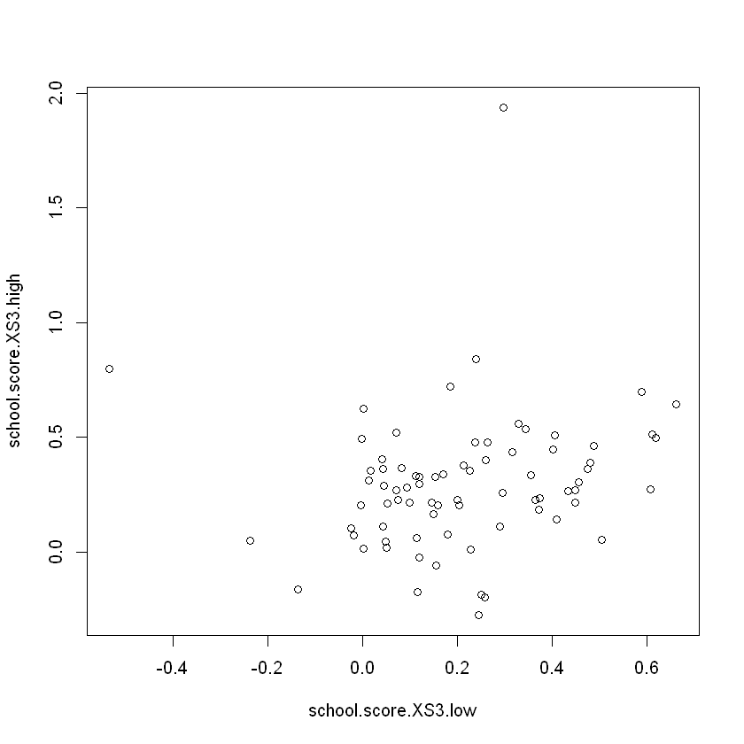
plot(school.score.XS3.low, school.score.XS3.high)
t.test(school.score.XS3.high - school.score.XS3.low)
	One Sample t-test

data:  school.score.XS3.high - school.score.XS3.low
t = 2.2326, df = 75, p-value = 0.02856
alternative hypothesis: true mean is not equal to 0
95 percent confidence interval:
 0.009188917 0.161400046
sample estimates:
 mean of x
0.08529448
The difference in means between high and low \(S3\) schools is statistically significant (p-value = 0.02856)
The provided scatter plot visualizes the relationship between the school scores for low and high \(S3\) values. Points in the plot represent schools, with their respective debiased scores for \(S3\) below 6 on the x-axis and for \(S3\) 6 or above on the y-axis.
Schools with higher \(S3\) values tend to have higher debiased scores, as indicated by the positive correlation in the scatter plot.
The formal tests for \(X1\) and \(X2\) reveal that \(X1\) has a statistically significant effect on the school scores, whereas \(X2\) does not. The ANOVA test for \(X2\) levels also shows no significant differences across levels. The formal test for \(S3\) indicates a statistically significant effect on the school scores, supported by the scatter plot visualizing the positive relationship.
2.4. Look at school-wise heterogeneity#
pardef = par(mar = c(5, 4, 4, 2) + 0.5, cex.lab=1.5, cex.axis=1.5, cex.main=1.5, cex.sub=1.5)
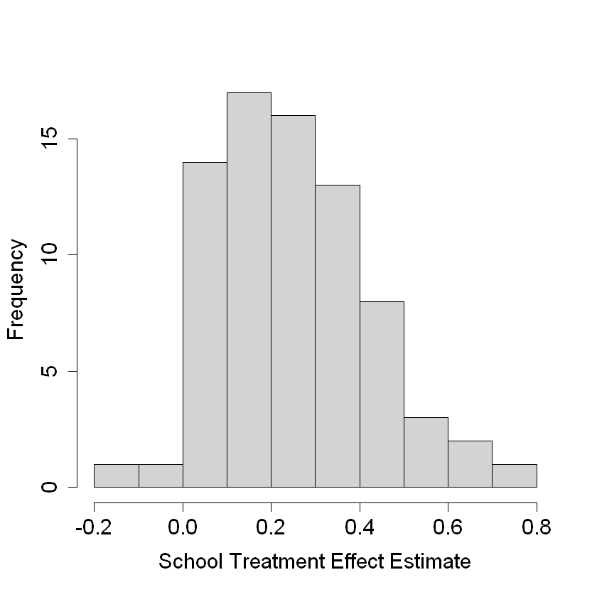
hist(school.score, xlab = "School Treatment Effect Estimate", main = "")
#
# Re-check ATE... sanity check only
#
ate.hat = mean(school.score)
se.hat = sqrt(var(school.score) / length(school.score - 1))
print(paste(round(ate.hat, 3), "+/-", round(1.96 * se.hat, 3)))
[1] "0.247 +/- 0.039"
#
# Look at variation in propensity scores
#

DF = X
DF$W.hat = cf$W.hat

pardef = par(mar = c(5, 4, 4, 2) + 0.5, cex.lab=1.5, cex.axis=1.5, cex.main=1.5, cex.sub=1.5)
boxplot(W.hat ~ S3, data = DF, ylab = "Propensity Score", xlab = "Student Expectation of Success")
lines(smooth.spline(X$S3, cf$W.hat), lwd = 2, col = 4)
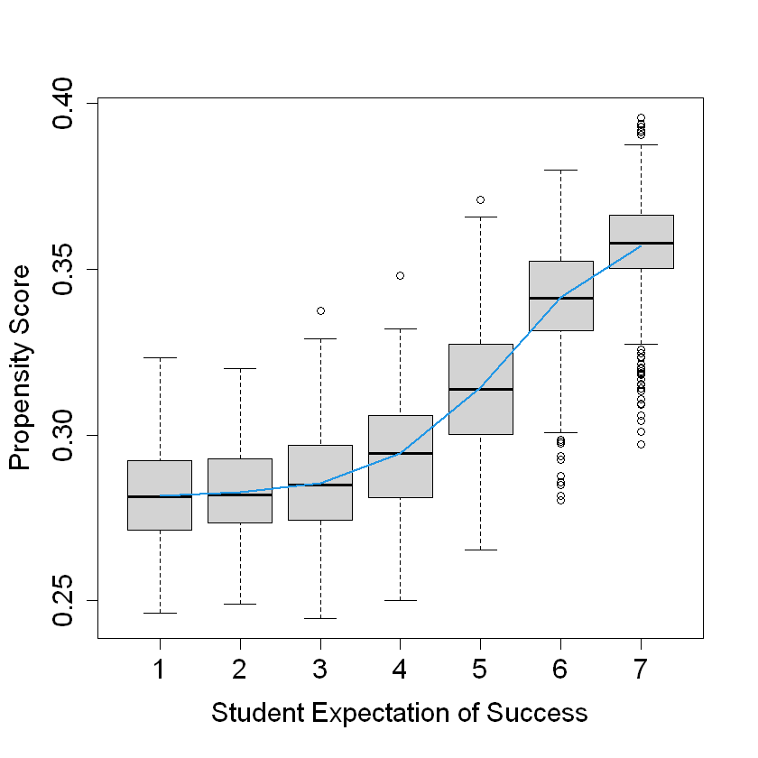
The boxplot shows the distribution of propensity scores for each level of student expectation of success (S3).
The smooth spline line shows an upward trend, indicating that propensity scores tend to increase with higher student expectations of success. This suggests that students with higher expectations of success are more likely to receive the treatment.
2.5. Analysis ignoring clusters. How do the results change?#
cf.noclust = causal_forest(X[,selected.idx], Y, W,
Y.hat = Y.hat, W.hat = W.hat,
tune.parameters = "all")
ATE.noclust = average_treatment_effect(cf.noclust)
paste("95% CI for the ATE:", round(ATE.noclust[1], 3),
"+/-", round(qnorm(0.975) * ATE.noclust[2], 3))
test_calibration(cf.noclust)
tau.hat.noclust = predict(cf.noclust)$predict
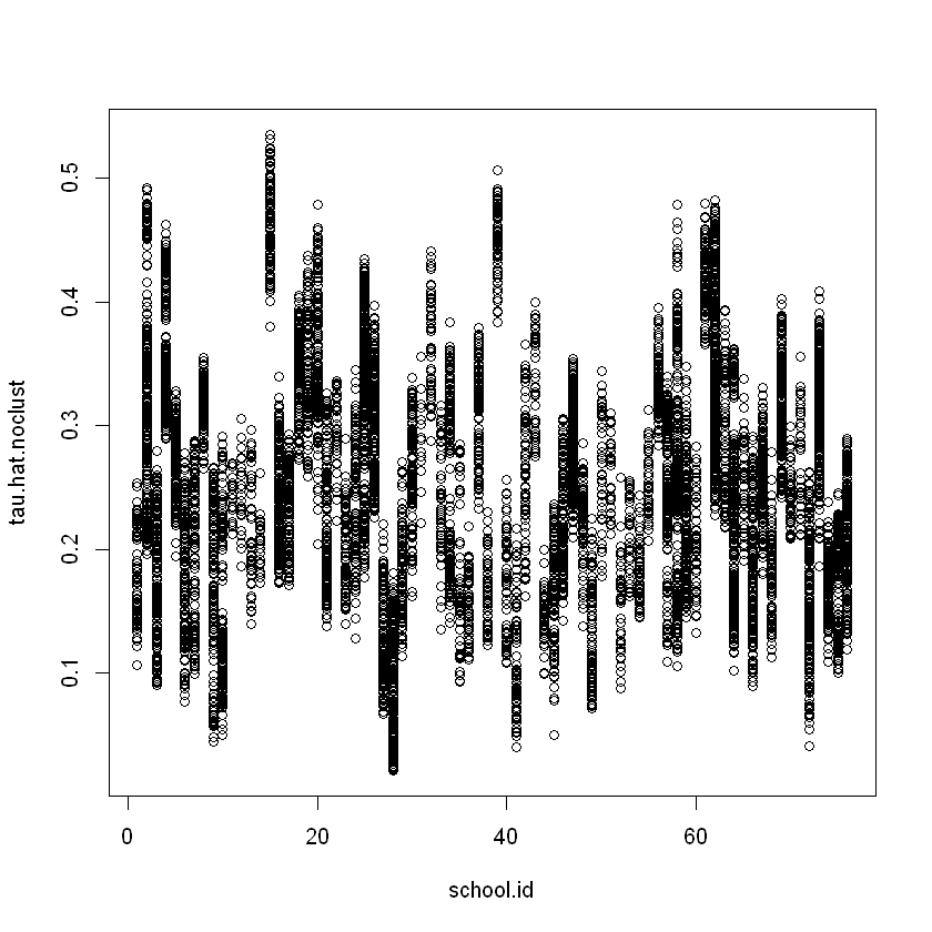
plot(school.id, tau.hat.noclust)
nfold = 5
school.levels = unique(school.id)
cluster.folds = sample.int(nfold, length(school.levels), replace = TRUE)
tau.hat.crossfold = rep(NA, length(Y))
for (foldid in 1:nfold) {
print(foldid)
infold = school.id %in% school.levels[cluster.folds == foldid]
cf.fold = causal_forest(X[!infold, selected.idx], Y[!infold], W[!infold],
Y.hat = Y.hat[!infold], W.hat = W.hat[!infold],
tune.parameters = "all")
pred.fold = predict(cf.fold, X[infold, selected.idx])$predictions
tau.hat.crossfold[infold] = pred.fold
}
cf.noclust.cpy = cf.noclust
cf.noclust.cpy$predictions = tau.hat.crossfold
cf.noclust.cpy$clusters = school.id
test_calibration(cf.noclust.cpy)
Rloss = mean(((Y - Y.hat) - tau.hat * (W - W.hat))^2)
Rloss.noclust = mean(((Y - Y.hat) - tau.hat.noclust * (W - W.hat))^2)
Rloss.crossfold = mean(((Y - Y.hat) - tau.hat.crossfold * (W - W.hat))^2)
c(Rloss.noclust - Rloss, Rloss.crossfold - Rloss)
summary(aov(dr.score ~ factor(school.id)))
Best linear fit using forest predictions (on held-out data)
as well as the mean forest prediction as regressors, along
with one-sided heteroskedasticity-robust (HC3) SEs:

                               Estimate Std. Error t value  Pr(>t)
mean.forest.prediction         1.007542   0.044966 22.4068 < 2e-16 ***
differential.forest.prediction 0.509010   0.123142  4.1335 1.8e-05 ***
---
Signif. codes:  0 '***' 0.001 '**' 0.01 '*' 0.05 '.' 0.1 ' ' 1
[1] 1
[1] 2
[1] 3
[1] 4
[1] 5
Best linear fit using forest predictions (on held-out data)
as well as the mean forest prediction as regressors, along
with one-sided heteroskedasticity-robust (HC3) SEs:

                               Estimate Std. Error t value  Pr(>t)
mean.forest.prediction         1.007637   0.065782  15.318 < 2e-16 ***
differential.forest.prediction 0.356911   0.229080   1.558 0.05963 .
---
Signif. codes:  0 '***' 0.001 '**' 0.01 '*' 0.05 '.' 0.1 ' ' 1
- 0.000113715565374151
- 0.000346614550637281
                     Df Sum Sq Mean Sq F value   Pr(>F)
factor(school.id)    75    200   2.673   1.989 8.85e-07 ***
Residuals         10315  13861   1.344
---
Signif. codes:  0 '***' 0.001 '**' 0.01 '*' 0.05 '.' 0.1 ' ' 1
2.6. Analysis without fitting the propensity score#
#
# Analaysis without fitting the propensity score
#
cf.noprop = causal_forest(X[,selected.idx], Y, W,
Y.hat = Y.hat, W.hat = mean(W),
tune.parameters = "all",
equalize.cluster.weights = TRUE,
clusters = school.id)
tau.hat.noprop = predict(cf.noprop)$predictions
ATE.noprop = average_treatment_effect(cf.noprop)
paste("95% CI for the ATE:", round(ATE.noprop[1], 3),
"+/-", round(qnorm(0.975) * ATE.noprop[2], 3))
pardef = par(mar = c(5, 4, 4, 2) + 0.5, cex.lab=1.5, cex.axis=1.5, cex.main=1.5, cex.sub=1.5)
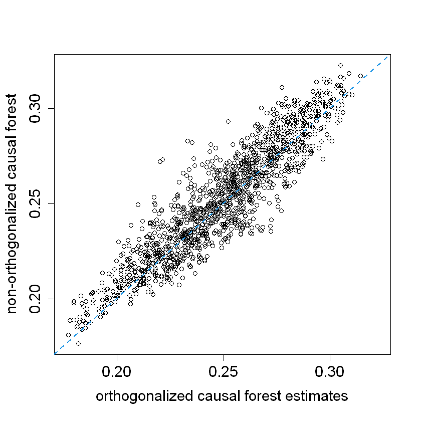
plot(tau.hat, tau.hat.noprop,
xlim = range(tau.hat, tau.hat.noprop),
ylim = range(tau.hat, tau.hat.noprop),
xlab = "orthogonalized causal forest estimates",
ylab = "non-orthogonalized causal forest")
abline(0, 1, lwd = 2, lty = 2, col = 4)
par = pardef
#
# Train forest on school-wise DR scores
#

school.X = (t(school.mat) %*% as.matrix(X[,c(4:8, 25:28)])) / school.size
school.X = data.frame(school.X)
colnames(school.X) = c("X1", "X2", "X3", "X4", "X5",
                    "XC.1", "XC.2", "XC.3", "XC.4")

dr.score = tau.hat + W / cf$W.hat * (Y - cf$Y.hat - (1 - cf$W.hat) * tau.hat) -
  (1 - W) / (1 - cf$W.hat) * (Y - cf$Y.hat + cf$W.hat * tau.hat)
school.score = t(school.mat) %*% dr.score / school.size

school.forest = regression_forest(school.X, school.score)
school.pred = predict(school.forest)$predictions
test_calibration(school.forest)


# Alternative OLS analysis
school.DF = data.frame(school.X, school.score=school.score)
coeftest(lm(school.score ~ ., data = school.DF), vcov = vcovHC)
Best linear fit using forest predictions (on held-out data)
as well as the mean forest prediction as regressors, along
with one-sided heteroskedasticity-robust (HC3) SEs:

                               Estimate Std. Error t value Pr(>t)
mean.forest.prediction         1.005143   0.082815 12.1373 <2e-16 ***
differential.forest.prediction 0.722757   0.657557  1.0992 0.1376
---
Signif. codes:  0 '***' 0.001 '**' 0.01 '*' 0.05 '.' 0.1 ' ' 1
t test of coefficients:

              Estimate Std. Error t value Pr(>|t|)
(Intercept)  0.2433855  0.0771666  3.1540 0.002424 **
X1          -0.0495439  0.0291700 -1.6985 0.094132 .
X2           0.0127040  0.0337703  0.3762 0.707984
X3           0.0093747  0.0264377  0.3546 0.724023
X4           0.0222932  0.0256041  0.8707 0.387080
X5          -0.0342604  0.0268506 -1.2760 0.206440
XC.1        -0.0030273  0.0930189 -0.0325 0.974136
XC.2         0.0839073  0.1051560  0.7979 0.427772
XC.3        -0.1351282  0.0878695 -1.5378 0.128871
XC.4         0.0398784  0.0820527  0.4860 0.628570
---
Signif. codes:  0 '***' 0.001 '**' 0.01 '*' 0.05 '.' 0.1 ' ' 1
2.7. The code plot six plots in the Make some plots section, so explain what you find there.#
pardef = par(mar = c(5, 4, 4, 2) + 0.5, cex.lab=1.5, cex.axis=1.5, cex.main=1.5, cex.sub=1.5)
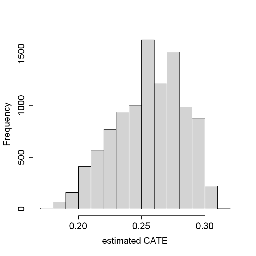
hist(tau.hat, xlab = "estimated CATE", main = "")
pardef = par(mar = c(5, 4, 4, 2) + 0.5, cex.lab=1.5, cex.axis=1.5, cex.main=1.5, cex.sub=1.5)
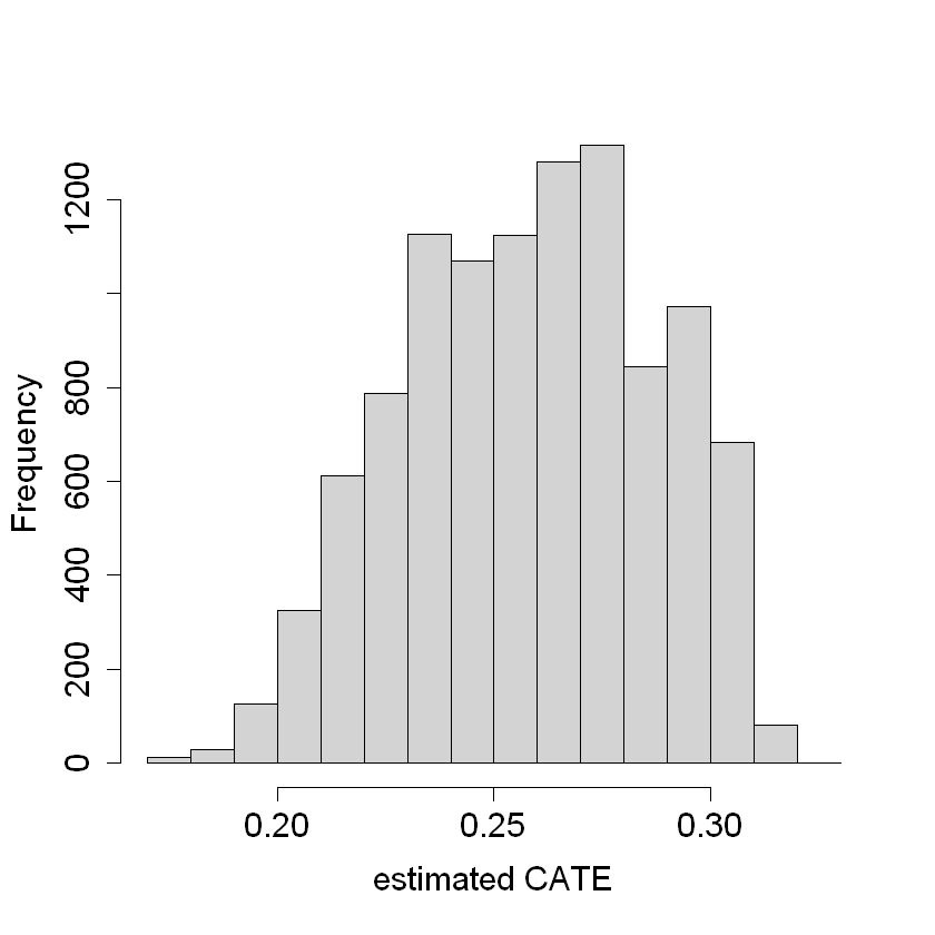
hist(tau.hat.noprop, xlab = "estimated CATE", main = "")
pardef = par(mar = c(5, 4, 4, 2) + 0.5, cex.lab=1.5, cex.axis=1.5, cex.main=1.5, cex.sub=1.5)
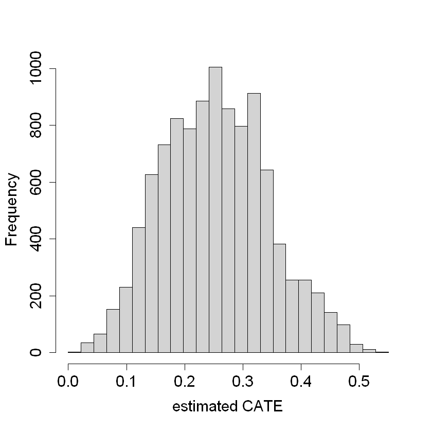
hist(tau.hat.noclust, xlab = "estimated CATE", main = "",
breaks = seq(-0.0, 0.55, by = 0.55 / 25))
pardef = par(mar = c(5, 4, 4, 2) + 0.5, cex.lab=1.5, cex.axis=1.5, cex.main=1.5, cex.sub=1.5)
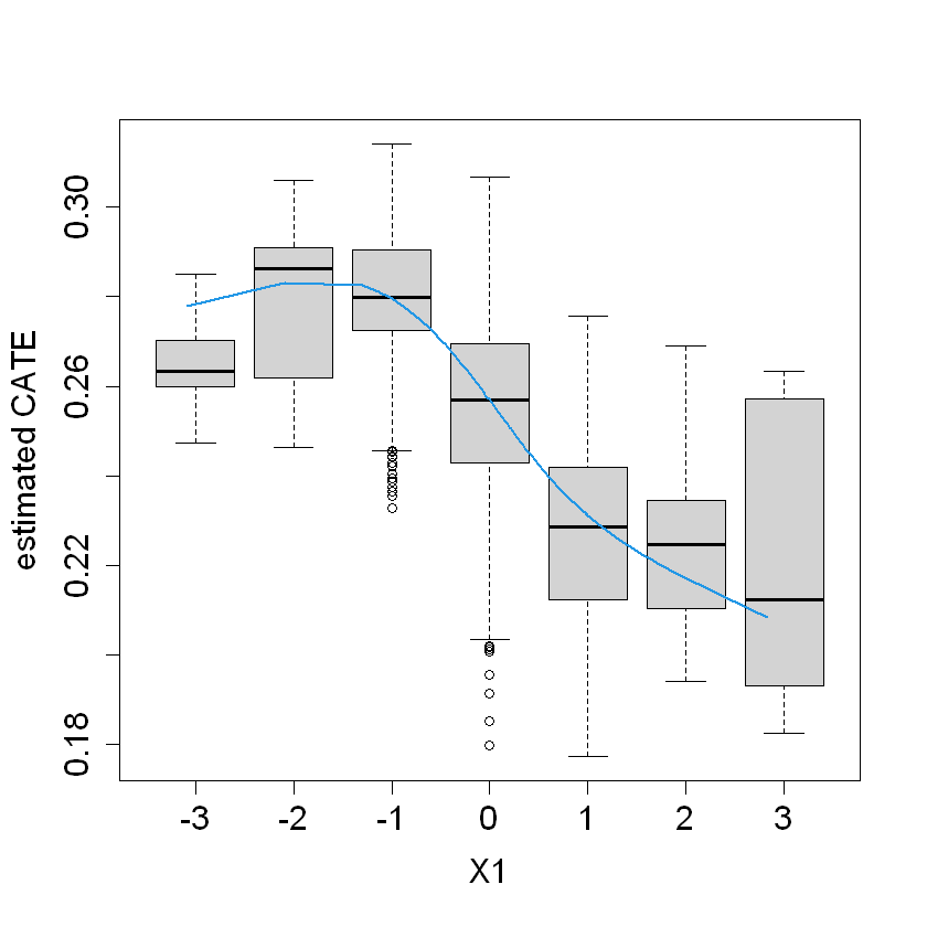
boxplot(tau.hat ~ round(X$X1), xlab = "X1", ylab = "estimated CATE")
lines(smooth.spline(4 + X[,"X1"], tau.hat, df = 4), lwd = 2, col = 4)
pardef = par(mar = c(5, 4, 4, 2) + 0.5, cex.lab=1.5, cex.axis=1.5, cex.main=1.5, cex.sub=1.5)
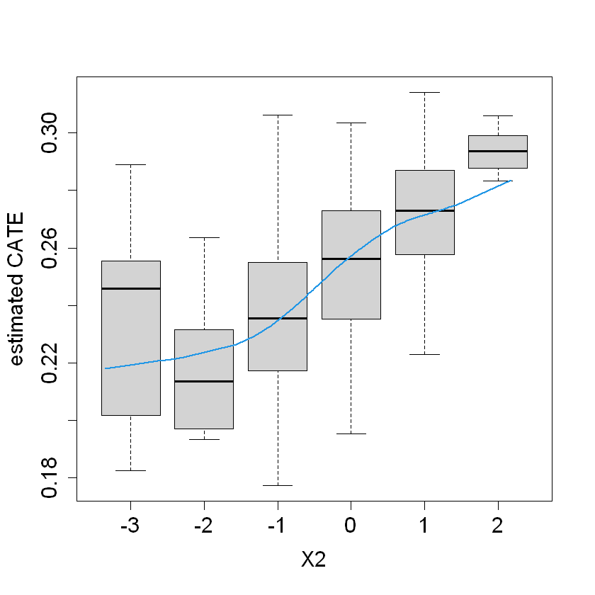
boxplot(tau.hat ~ round(X$X2), xlab = "X2", ylab = "estimated CATE")
lines(smooth.spline(4 + X[,"X2"], tau.hat, df = 4), lwd = 2, col = 4)
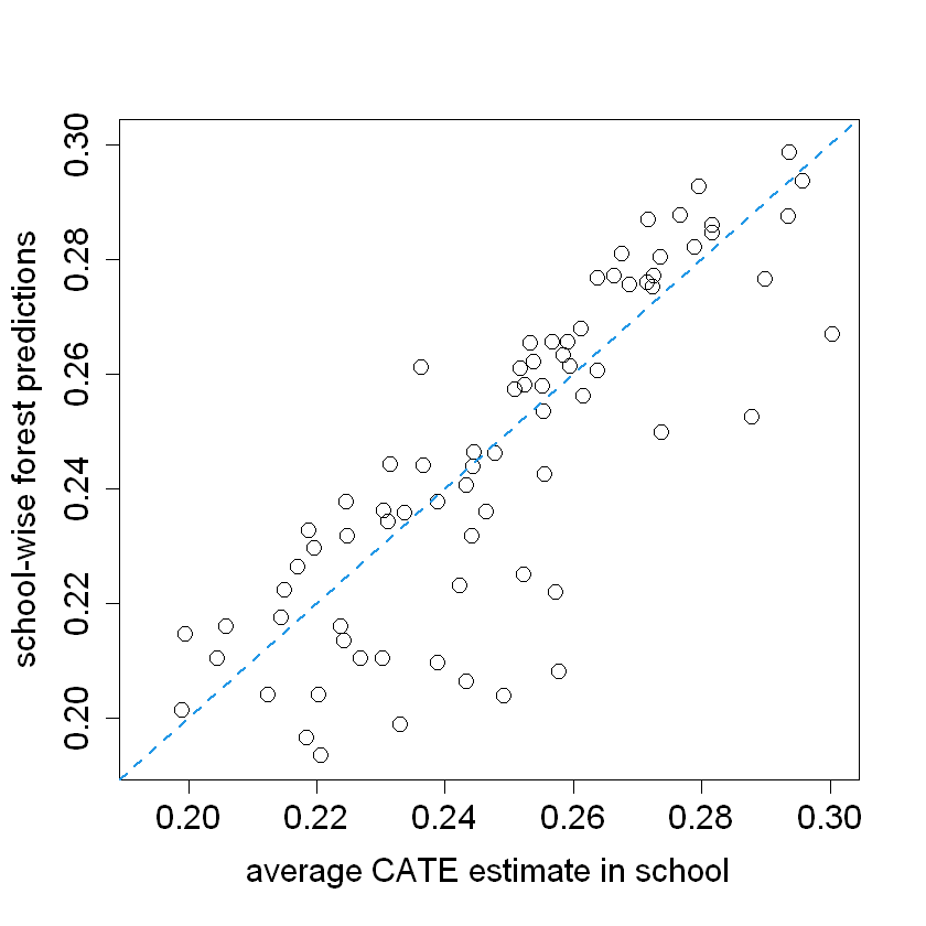
school.avg.tauhat = t(school.mat) %*% tau.hat / school.size
pardef = par(mar = c(5, 4, 4, 2) + 0.5, cex.lab=1.5, cex.axis=1.5, cex.main=1.5, cex.sub=1.5)
plot(school.avg.tauhat, school.pred, cex = 1.5,
xlim = range(school.avg.tauhat, school.pred),
ylim = range(school.avg.tauhat, school.pred),
xlab = "average CATE estimate in school",
ylab = "school-wise forest predictions")
abline(0, 1, lwd = 2, lty = 2, col = 4)
par = pardef
#
# Experiment with no orthogonalization
#
n.synth = 1000
p.synth = 10
X.synth = matrix(rnorm(n.synth * p.synth), n.synth, p.synth)
W.synth = rbinom(n.synth, 1, 1 / (1 + exp(-X.synth[,1])))
Y.synth = 2 * rowMeans(X.synth[,1:6]) + rnorm(n.synth)
Y.forest.synth = regression_forest(X.synth, Y.synth)
Y.hat.synth = predict(Y.forest.synth)$predictions
W.forest.synth = regression_forest(X.synth, W.synth)
W.hat.synth = predict(W.forest.synth)$predictions
cf.synth = causal_forest(X.synth, Y.synth, W.synth,
Y.hat = Y.hat.synth, W.hat = W.hat.synth)
ATE.synth = average_treatment_effect(cf.synth)
paste("95% CI for the ATE:", round(ATE.synth[1], 3),
"+/-", round(qnorm(0.975) * ATE.synth[2], 3))
cf.synth.noprop = causal_forest(X.synth, Y.synth, W.synth,
Y.hat = Y.hat.synth, W.hat = mean(W.synth))
ATE.synth.noprop = average_treatment_effect(cf.synth.noprop)
paste("95% CI for the ATE:", round(ATE.synth.noprop[1], 3),
"+/-", round(qnorm(0.975) * ATE.synth.noprop[2], 3))
2.8. Visualize school-level covariates by treatment heterogeneity#
This section aims to visualize how different school-level covariates (features) vary across different levels of estimated treatment heterogeneity. Specifically, it divides the schools into terciles (three groups) based on their predicted treatment effects and examines the standardized mean values of covariates within each tercile.
#
# Visualize school-level covariates by treatment heterogeneity
#

school.X.std = scale(school.X)
school.tercile = cut(school.pred,
                     breaks = c(-Inf, quantile(school.pred, c(1/3, 2/3)), Inf))
school.tercile.mat = model.matrix(~ school.tercile + 0)
school.means = diag(1 / colSums(school.tercile.mat)) %*% t(school.tercile.mat) %*% as.matrix(school.X.std)

MM = max(abs(school.means))
HC = heat.colors(21)
school.col = apply(school.means, 1:2, function(aa) HC[1 + round(20 * (0.5 + aa))])

DF.plot = data.frame(tercile=rep(factor(1:3, labels=c("low", "mid", "high")), 9), mean=as.numeric(school.means),
                     feature = factor(rbind(colnames(school.X), colnames(school.X), colnames(school.X))))

ggplot(data = DF.plot, aes(x = feature, y = tercile, fill = mean)) +
    geom_tile() + scale_fill_gradient(low = "white", high = "steelblue") +
    theme(axis.text = element_text(size=12), axis.title = element_text(size=14),
          legend.title = element_text(size=14), legend.text = element_text(size=12)) +
    theme(panel.background = element_blank())

mean(school.X$XC.3)
mean(school.X$XC.3[as.numeric(school.tercile) == 1])
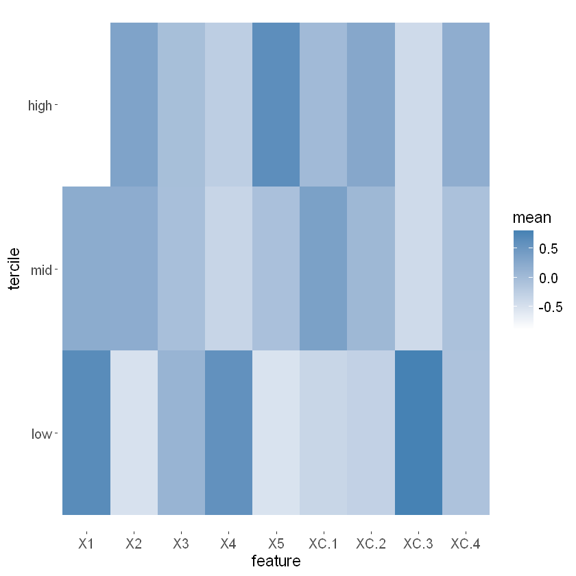
The heatmap reveals the relationship between school-level covariates and predicted treatment effects. Certain covariates (e.g., X1, X4, and XC.3) exhibit distinct patterns across the terciles, indicating their potential influence on treatment heterogeneity.
The analysis helps identify which covariates are more prevalent in schools with higher or lower treatment effects, providing insights into the factors driving the effectiveness of interventions across different schools.
2.9. CATE by school#
This section examines the Conditional Average Treatment Effects (CATE) for each school and visualizes how these estimates compare to the average CATE predictions.
ord = order(order(school.pred))
school.sort = ord[school.id]


pardef = par(mar = c(5, 4, 4, 2) + 0.5, cex.lab=1.5, cex.axis=1.5, cex.main=1.5, cex.sub=1.5)
boxplot(tau.hat.noclust ~ school.sort, xaxt = "n",
        xlab = "school", ylab = "estimated CATE")
points(1:76, sort(school.pred), col = 4, pch = 16)
legend("topleft", c("school mean CATE", "CATE w/o clustering"), pch = c(16, 1), col = c(4, 1), cex = 1.5)
par = pardef
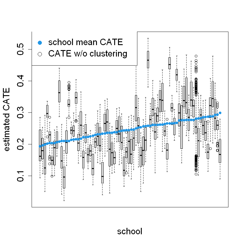
There is substantial heterogeneity in the treatment effects across different schools, as indicated by the range of CATE values within each boxplot. This suggests that the impact of the treatment varies significantly between schools
The clustering approach seems to provide more stable estimates of the treatment effect for each school, as evidenced by the smaller spread in the mean CATE points compared to the CATE w/o clustering